
LSA Types 1,2 and 3
OSPF learns the topology by exchanging link-state advertisements (LSAs). Engineers preparing for the CCNA exam are often intimidated by the LSA concept and either do not invest enough time to understand it fully or skip it altogether. However, understanding the different types of LSAs leads to a better understanding of the protocol operation. In this lesson, we explain LSA Types 1, 2, and 3 in an easily understandable way.
What are the main building blocks of an OSPF area?
Let’s look at the basic topology shown in the diagram below, which we are going to use as a context in the upcoming LSA examples. What are the two building blocks of the topology that you can clearly distinguish?
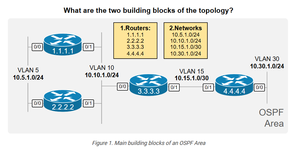
In the context of a routing protocol, the topology includes two main components: routers with links and networks between the routers. Well, these are the first two LSA types that OSPF uses to build the topology inside an area:
- LSA Type 1 (called Router LSA) for each device in the area.
- LSA Type 2 (called Network LSA) for each network with an elected DR and at least one neighbor.
Let’s walk through each link-state advertisement type in more detail and see how it fits in the bigger picture.
LSA Type 1 – Router LSA
Every OSPF device creates a Router LSA for itself and sends it to all neighbors inside the area, as shown in the diagram below. The LSA is flooded until every device in the area has a copy.
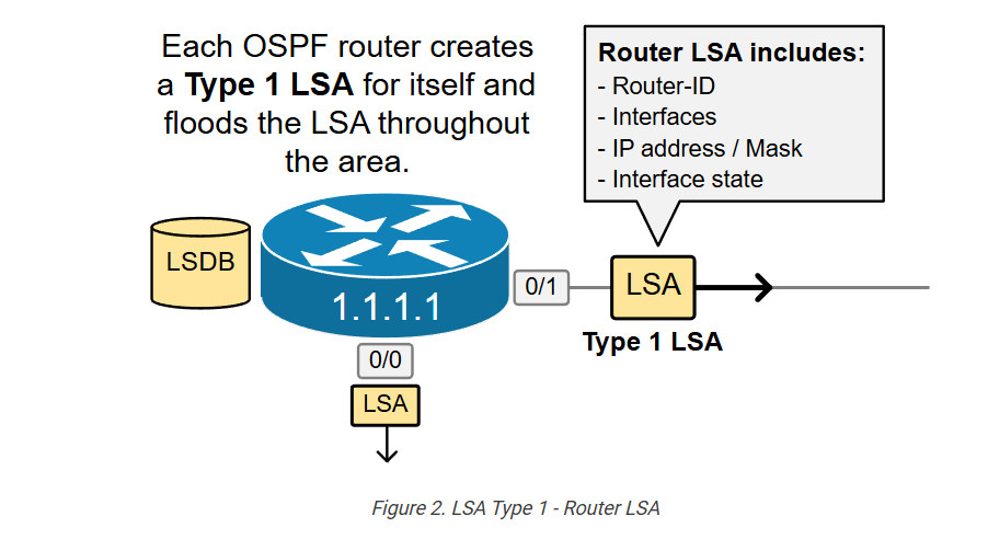
The Router LSA is uniquely identified by the RID of the originating device and includes the following information:
- The RID.
- The router’s own interfaces.
- IP addresses / Mask.
- Cost of the interface.
- Current interface status.
Every OSPF device creates and floods its own Router LSA inside the area, ensuring that all devices know the same LSAs. In other words, the process ensures that everyone inside an area knows about every OSPF device and its links, as shown in the diagram below.
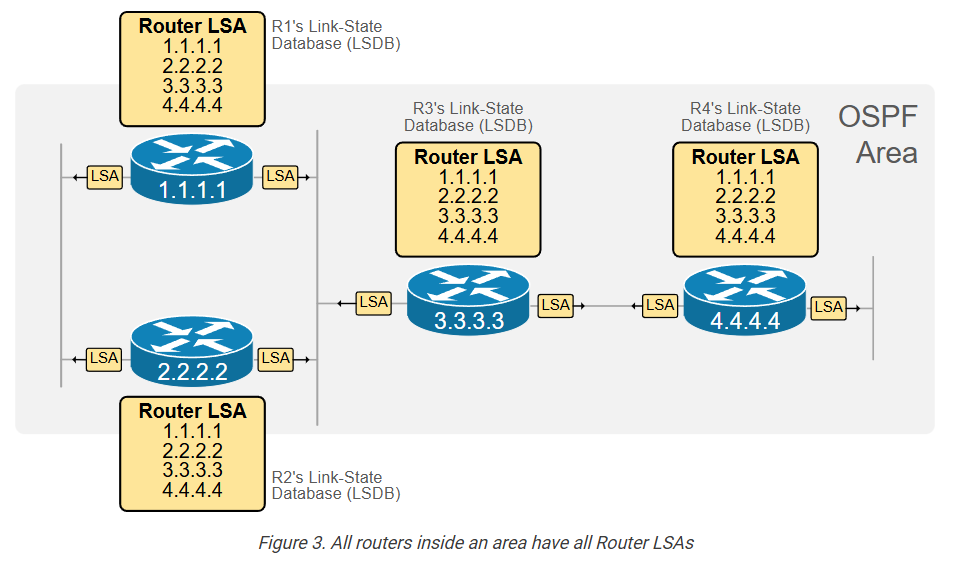
Notice that the link-state database (LSDB) of every device in the area contains one Router LSA per device.
Router LSA – Show Commands
Now, to fully understand the Router LSA concept, let’s reconstruct the topology only by looking at one of the router’s link-state databases (LSDB). Since all devices are in the same area, they have identical LSDB databases, so it doesn’t matter which one we are looking at.
Let’s assume that we know nothing about the topology.
First, using the show ip ospf database command, we can see a summary of all router LSAs. It shows us that there are four devices in the area, which is actually Area 0, as highlighted in blue.
					R1# sh ip ospf database

            OSPF Router with ID (1.1.1.1) (Process ID 1)

                Router Link States (Area 0)
Link ID         ADV Router      Age         Seq#       Checksum Link count
1.1.1.1         1.1.1.1         1567        0x80000016 0x005052 2
2.2.2.2         2.2.2.2         1560        0x80000018 0x00286E 2
3.3.3.3         3.3.3.3         580         0x8000001B 0x00EE64 3
4.4.4.4         4.4.4.4         581         0x80000010 0x0087D7 3

                Net Link States (Area 0)
Link ID         ADV Router      Age         Seq#       Checksum
10.5.1.2        2.2.2.2         1576        0x80000001 0x00FB18
10.10.1.3       3.3.3.3         1573        0x80000002 0x0044B4
So, we first learn that Area 0 has 4 routers. Okay, now let’s look at each router LSA in detail.
Using the following command, we check the content of R1’s router LSA. Let’s see what information it can give us.
					R1# show ip ospf database router 1.1.1.1

            OSPF Router with ID (1.1.1.1) (Process ID 1)

                Router Link States (Area 0)

  LS age: 1771
  Options: (No TOS-capability, DC)
  LS Type: Router Links
  Link State ID: 1.1.1.1
  Advertising Router: 1.1.1.1
  LS Seq Number: 80000016
  Checksum: 0x5052
  Length: 48
  Number of Links: 2
    Link connected to: a Transit Network
     (Link ID) Designated Router address: 10.10.1.3
     (Link Data) Router Interface address: 10.10.1.1
      Number of MTID metrics: 0
       TOS 0 Metrics: 10
    Link connected to: a Transit Network
     (Link ID) Designated Router address: 10.5.1.2
     (Link Data) Router Interface address: 10.5.1.1
      Number of MTID metrics: 0
       TOS 0 Metrics: 10
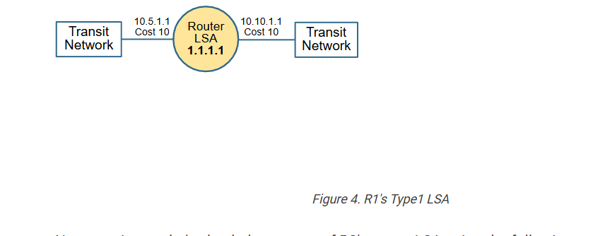
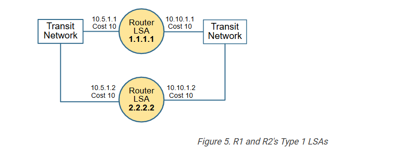
We can learn that R1 has two interfaces that connect to two “Transit Networks.” We can also see the IP addresses of each interface and the OSPF cost. Therefore, we can reconstruct the following topology from the information we have just learned.
Now, moving on, let’s check the context of R2’s router LSA using the following command.
					R1# show ip ospf database router 2.2.2.2

            OSPF Router with ID (1.1.1.1) (Process ID 1)

                Router Link States (Area 0)
  LS age: 354
  Options: (No TOS-capability, DC)
  LS Type: Router Links
  Link State ID: 2.2.2.2
  Advertising Router: 2.2.2.2
  LS Seq Number: 8000001F
  Checksum: 0x1A75
  Length: 48
  Number of Links: 2

    Link connected to: a Transit Network
     (Link ID) Designated Router address: 10.10.1.3
     (Link Data) Router Interface address: 10.10.1.2
      Number of MTID metrics: 0
       TOS 0 Metrics: 10
    Link connected to: a Transit Network
     (Link ID) Designated Router address: 10.5.1.2
     (Link Data) Router Interface address: 10.5.1.2
      Number of MTID metrics: 0
       TOS 0 Metrics: 10
We learned that R2 also has two interfaces connected to the same two transit networks. We learned the IP addresses and cost of each interface. Therefore, we can draw the following diagram from the information we’ve got so far.
Moving on, let’s check the R3 database.
					R1# show ip ospf database router 3.3.3.3

            OSPF Router with ID (1.1.1.1) (Process ID 1)

                Router Link States (Area 0)
  LS age: 1193
  Options: (No TOS-capability, DC)
  LS Type: Router Links
  Link State ID: 3.3.3.3
  Advertising Router: 3.3.3.3
  LS Seq Number: 80000021
  Checksum: 0xE26A
  Length: 60
  Number of Links: 3

    Link connected to: another Router (point-to-point)
     (Link ID) Neighboring Router ID: 4.4.4.4
     (Link Data) Router Interface address: 10.15.1.1
      Number of MTID metrics: 0
       TOS 0 Metrics: 10
    Link connected to: a Stub Network
     (Link ID) Network/subnet number: 10.15.1.0
     (Link Data) Network Mask: 255.255.255.252
      Number of MTID metrics: 0
       TOS 0 Metrics: 10
    Link connected to: a Transit Network
     (Link ID) Designated Router address: 10.10.1.3
     (Link Data) Router Interface address: 10.10.1.3
      Number of MTID metrics: 0
       TOS 0 Metrics: 10
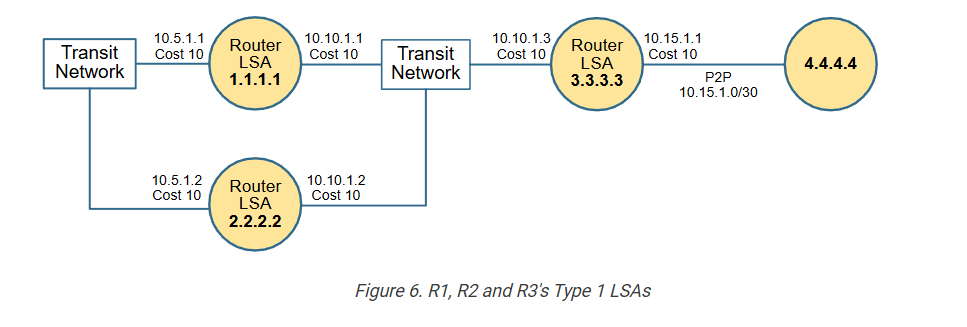
The first two links represent the point-to-point connection to R4. Since the interface is configured with the ip ospf network point-to-point command, it is not a multiaccess interface, and that’s why the output is different.
From the first link section, we can learn that this is a point-to-point connection that connects to neighbor 4.4.4.4. From the second link section, we learn the IP address / Mask of the P2P link. The third link section shows that R3 also connects to the transit network that R1 and R2 connect to.
Therefore, we can draw the following diagram from the information we have collected so far.
Lastly, let’s check the link-state information of R4.
					R1# show ip ospf database router 4.4.4.4

            OSPF Router with ID (1.1.1.1) (Process ID 1)

                Router Link States (Area 0)
  LS age: 1397
  Options: (No TOS-capability, DC)
  LS Type: Router Links
  Link State ID: 4.4.4.4
  Advertising Router: 4.4.4.4
  LS Seq Number: 80000016
  Checksum: 0x7BDD
  Length: 60
  Number of Links: 3

    Link connected to: another Router (point-to-point)
     (Link ID) Neighboring Router ID: 3.3.3.3
     (Link Data) Router Interface address: 10.15.1.2
      Number of MTID metrics: 0
       TOS 0 Metrics: 10
    Link connected to: a Stub Network
     (Link ID) Network/subnet number: 10.15.1.0
     (Link Data) Network Mask: 255.255.255.252
      Number of MTID metrics: 0
       TOS 0 Metrics: 10
    Link connected to: a Stub Network
     (Link ID) Network/subnet number: 10.30.1.0
     (Link Data) Network Mask: 255.255.255.0
      Number of MTID metrics: 0
       TOS 0 Metrics: 10
Notice that R4 has a point-to-point link connecting to R3. The second link represents the P2P subnet, and the third link is a different connection to a “Stub Network” 10.30.1.0/24.
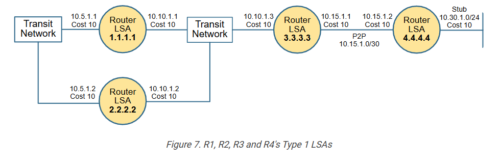
We were able to reconstruct the entire topology by only using the information from the Type 1 LSAs in the link-state database of R1. If we compare the diagram above with the one in Figure 1, we can see they are pretty much the same. However, why then do we need to have LSA Type 2? – Because there is a problem we need to discuss.
LSA Type 2 – Network LSA
OSPF uses an additional Link-state Advertisement Type 2 (called Network LSA) to construct multiaccess network segments like Ethernet VLAN.
					R1# sh ip ospf database

            OSPF Router with ID (1.1.1.1) (Process ID 1)

                Router Link States (Area 0)
Link ID         ADV Router      Age         Seq#       Checksum Link count
1.1.1.1         1.1.1.1         832         0x8000001D 0x004259 2
2.2.2.2         2.2.2.2         941         0x8000001F 0x001A75 2
3.3.3.3         3.3.3.3         1709        0x80000021 0x00E26A 3
4.4.4.4         4.4.4.4         1816        0x80000016 0x007BDD 3

                Net Link States (Area 0)
Link ID         ADV Router      Age         Seq#       Checksum
10.5.1.2        2.2.2.2         941         0x80000008 0x00ED1F
10.10.1.3       3.3.3.3         698         0x80000009 0x0036BB
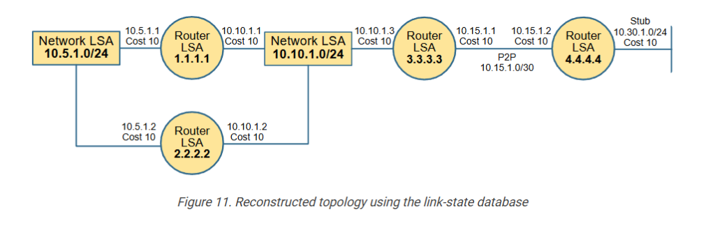
In Type 1 Link-State Advertisement, there are two types of multiaccess networks – a “Transit Network” and a “Stub Network”:
- A Transit network in OSPF is a network that can carry data between different OSPF routers. Essentially, it’s a network segment that has a DR and at least one more OSPF neighbor. For example, transit networks in our topology are 10.5.1.0/24 and 10.10.1.0/24.
- A Stub network in OSPF does not forward traffic between OSPF routers. It only hosts endpoints directly connected to a single OSPF device, meaning it’s a dead-end from the perspective of OSPF routing. For example, a stub network in our topology is 10.30.1.0/24.
When a multi-access segment is represented as a Transit Network, it means that an LSA Type 2 exists that lists all OSPF routers that connect to that segment. Let’s see why.
But why does OSPF need LSA Type 2?
Using the Router LSAs, we figured out that R1, R2, and R3 connect to a “Transit Network”, as shown in the diagram below. But how can we be 100% sure that the three routers really connect to the same multiaccess segment – for example, to the same VLAN? Looking at the information available in the Router LSAs, can you be 100% sure? No, you can’t be.
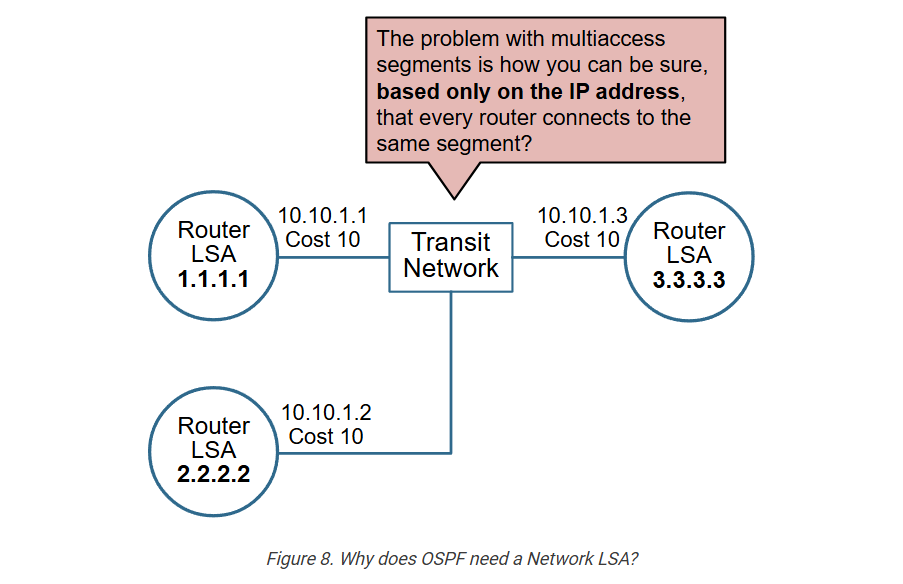
We concluded that all three routers connect to the same segment because they have IP addresses from the same network – R1 has 10.10.1.1, R2 has 10.10.1.2, and R3 has 10.10.1.3. But is this undeniable proof that they connect to the same VLAN?
No, it is not. The routers may be connected, as shown in the diagram below. Purely based on the IP addresses, you can’t be sure whether they connect to the same multi-access network.
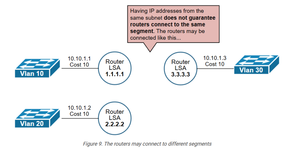
That’s why OSPF needs an additional link-state type that proves whether routers connect to the same multiaccess network. Otherwise, the routing process could create traffic black holes.
How does the Network LSA solve the problem?
First, recall that on multiaccess networks such as a traditional Ethernet VLAN, OSPF routers elect a Designated Router (DR) and a Backup Designated Router (BDR) and establish full adjacency only with the DR and the BDR. If you don’t know or recall what DR/BDR is, check out our OSPF DR and BDR lesson.
The DR on any multiaccess segment can undeniably tell which routers connect to that segment because it establishes a full OSPF adjacency with them (which implies they have connectivity and exchange packets). Using this logic, the DR advertises an LSA Type 2, which lists all connected routers, as shown in the diagram below.
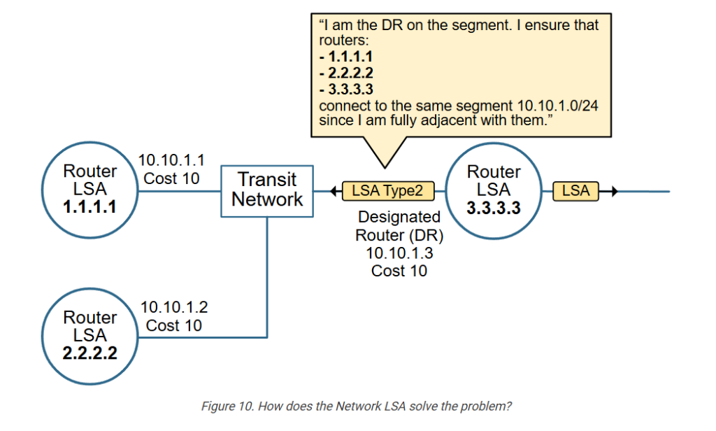
This technique ensures that the topology reconstructed from the information in the Link-state Database is accurate and represents the actual physical connectivity.
In our example topology, there are two Transit Networks – 10.5.1.0/24 and 10.10.1.0/24. R3’s interface 10.10.1.3 is the DR for network 10.10.1.0/24. If we look at the Network LSA that R3 creates and floods for that network, we can see the three routers that connect to the segment (highlighted in blue).
					R1# sh ip ospf database network 10.10.1.3

            OSPF Router with ID (1.1.1.1) (Process ID 1)

                Net Link States (Area 0)
  LS age: 800
  Options: (No TOS-capability, DC)
  LS Type: Network Links
  Link State ID: 10.10.1.3 (address of Designated Router)
  Advertising Router: 3.3.3.3
  LS Seq Number: 80000009
  Checksum: 0x36BB
  Length: 36
  Network Mask: /24
        Attached Router: 3.3.3.3
        Attached Router: 1.1.1.1
        Attached Router: 2.2.2.2
R3 knows for sure that the three routers actually connect to the same network because it maintains full OSPF adjacency with them over the VLAN.
					R3# sh ip ospf neighbor

Neighbor ID     Pri   State           Dead Time   Address         Interface
4.4.4.4           0   FULL/  -        00:00:36    10.15.1.2       Ethernet0/1
1.1.1.1           1   FULL/DROTHER    00:00:37    10.10.1.1       Ethernet0/0
2.2.2.2           1   FULL/BDR        00:00:39    10.10.1.2       Ethernet0/0
We can make the same check for the other transit network, 10.5.1.0/24, using the link-state database of any of the devices. In the end, we can construct the actual topology as shown in the diagram below.
Notice the following aspects of the process of creating and advertising a LSA Type 2:
- If a multiaccess interface has no neighbors, it is listed as “Stub Network” in the LSA Type 1 and does not require LSA Type 2. For example, this is the case for 10.30.1.0/24 connected to R4.
- If a multiaccess interface has at least one neighbor, it is listed as “Transit Network” in the LSA Type 1, which means a Type 2 LSA exists that further describes that network.
- Only the DR floods a Network LSA for the network because it has a full adjacency with all other OSPF devices on that multiaccess segment.
LSA Types 1 and 2 are enough to describe the topology inside a single OSPF Area. However, if the network has multiple areas, the routing process needs an additional link-state advertisement type to describe the networks in remote areas. Let’s see how it works.
LSA Type 3 – Summary LSA
You have seen by now that OSPF uses the area concept to break down a large network into smaller portions, reducing the size of the LSDB database. A smaller LSDB requires less RAM and CPU, making the network more efficient and scale better.
But how exactly does the concept of areas reduce the size of the LSDB?
LSAs Type 1 and 2 are local to an OSPF area. Area Border Routers (ABRs) do not forward LSAs Type 1 and 2 between areas, as shown in the diagram below.
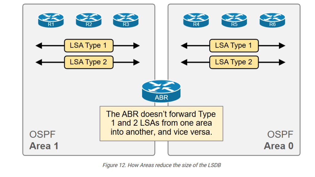
This results in a smaller link-state database per area, which optimizes the memory and CPU consumption of the OSPF process. However, routers still need to be able to reach networks in other areas.
Instead of having all devices across the entire network know all Type 1 and Type 2 LSAs, area border routers generate a Summary LSA that summarizes
What is LSA Type 3?
When a router connects two OSPF areas, it is called an Area Border Router (ABR). The ABR generates an LSA Type 3 for each subnet in one area and advertises each Type 3 LSA to the other area, as shown in the diagram below.
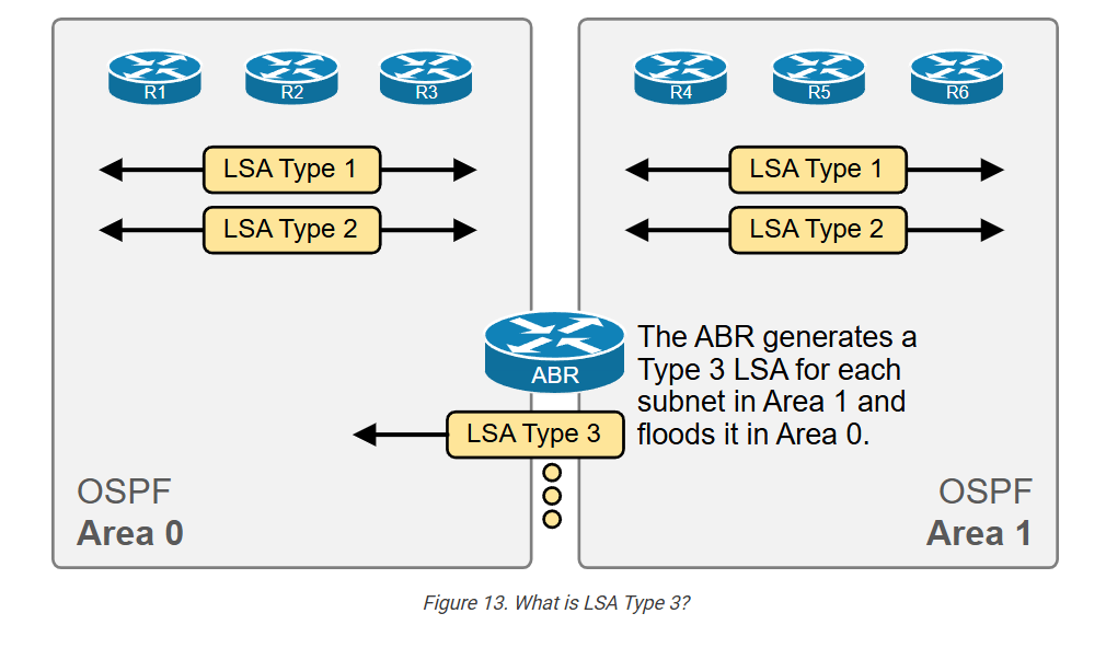
For example, suppose we have 5 subnets in Area 1. The ABR that connects Area 1 to Area 0 generates five LSA Type 3 and floods them into Area 0. Each LSA Type 3 represents one of the subnets in Area 1.
The Type 3 LSA does not contain any detailed topology information, such as link and cost. It just informs the routers inside the area that they can reach a particular subnet via the area border router. Hence, it is called a Summary LSA because the information inside is sparse compared to LSA Types 1 and 2.
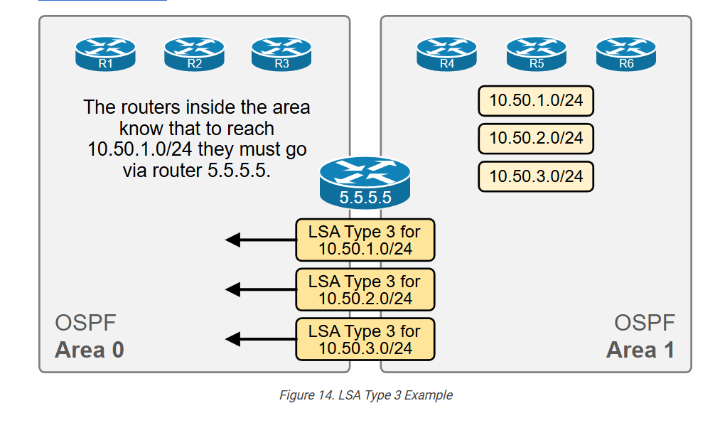
Let’s look at the example shown in the diagram above. Area 1 has three subnets (highlighted in yellow). The area border router 5.5.5.5 creates an LSA Type 3 for each subnet and floods it into Area 0.
Let’s check the LSDB of a router in Area 0 and see the Type 3 LSAs highlighted in blue.
					R1# sh ip ospf database

            OSPF Router with ID (1.1.1.1) (Process ID 1)

                Router Link States (Area 0)
Link ID         ADV Router      Age         Seq#       Checksum Link count
1.1.1.1         1.1.1.1         600         0x8000000C 0x006448 2
2.2.2.2         2.2.2.2         594         0x8000000D 0x003E63 2
3.3.3.3         3.3.3.3         537         0x8000000D 0x000B56 3
4.4.4.4         4.4.4.4         329         0x80000009 0x0050E5 3
5.5.5.5         5.5.5.5         235         0x80000007 0x007131 1

                Net Link States (Area 0)
Link ID         ADV Router      Age         Seq#       Checksum
10.5.1.2        2.2.2.2         594         0x80000005 0x00F31C
10.10.1.3       3.3.3.3         537         0x80000006 0x003CB8
10.30.1.4       4.4.4.4         329         0x80000005 0x008351

                Summary Net Link States (Area 0)
Link ID         ADV Router      Age         Seq#       Checksum
10.50.1.0       5.5.5.5         235         0x80000005 0x000DD9
10.50.2.0       5.5.5.5         235         0x80000005 0x0002E3
Let’s check the details of one of the Summary LSAs. Pay attention to the command used.
					R1# sh ip ospf database summary 10.50.1.0

            OSPF Router with ID (1.1.1.1) (Process ID 1)

                Summary Net Link States (Area 0)
  LS age: 398
  Options: (No TOS-capability, DC, Upward)
  LS Type: Summary Links(Network)
  Link State ID: 10.50.1.0 (summary Network Number)
  Advertising Router: 5.5.5.5
  LS Seq Number: 80000005
  Checksum: 0xDD9
  Length: 28
  Network Mask: /24
        MTID: 0  Metric: 1
Notice that the LSID is the network’s subnet address. The advertising router is the ABR 5.5.5.5. The subnet mask is /24, and the cost is 1. There is not much else we can find in the LSA Type 3. That’s why it is called a Summary LSA.
Notice that the routes a router learns via LSA Type 3 are inserted in the routing table as “O IA,” which stands for Inter-Area routes. (Routes from another area which are reachable via an ABR).
					R1# sh ip route
Codes: L - local, C - connected, S - static, R - RIP, M - mobile, B - BGP
       D - EIGRP, EX - EIGRP external, O - OSPF, IA - OSPF inter area
       N1 - OSPF NSSA external type 1, N2 - OSPF NSSA external type 2
       E1 - OSPF external type 1, E2 - OSPF external type 2, m - OMP
       n - NAT, Ni - NAT inside, No - NAT outside, Nd - NAT DIA
       i - IS-IS, su - IS-IS summary, L1 - IS-IS level-1, L2 - IS-IS level-2
       ia - IS-IS inter area, * - candidate default, U - per-user static route
       H - NHRP, G - NHRP registered, g - NHRP registration summary
       o - ODR, P - periodic downloaded static route, l - LISP
       a - application route
       + - replicated route, % - next hop override, p - overrides from PfR
       & - replicated local route overrides by connected

Gateway of last resort is not set

      10.0.0.0/8 is variably subnetted, 11 subnets, 3 masks
C        10.5.1.0/24 is directly connected, Ethernet0/0
L        10.5.1.1/32 is directly connected, Ethernet0/0
C        10.10.1.0/24 is directly connected, Ethernet0/1
L        10.10.1.1/32 is directly connected, Ethernet0/1
O        10.15.1.0/30 [110/20] via 10.10.1.3, 02:41:24, Ethernet0/1
O        10.30.1.0/24 [110/30] via 10.10.1.3, 02:41:24, Ethernet0/1
O IA     10.50.1.0/24 [110/31] via 10.10.1.3, 02:35:54, Ethernet0/1
O IA     10.50.2.0/24 [110/31] via 10.10.1.3, 02:35:54, Ethernet0/1
We still haven’t answered the most important question about OSPF Type 3 LSAs.
Why doesn’t OSPF use LSA type 1 and 2 between areas instead of Type 3?
Many engineers can’t answer this question even at the CCNP/CCIE level because they do not fully understand the concept.
OSPF uses LSA types 1 and 2 to build the topology inside an area. Every router describes itself and its links using LSA Type 1, while every DR describes a multiaccess segment and its connected devices. LSAs types 1 and 2 are enough for the SPF algorithm to calculate the best path to every network inside the area.
When an LSA Type 1 or LSA Type 2 changes, all routers inside the area must execute the SPF algorithm because the change impacts the choice of best routes. Running the SPF is a resource-intensive task requiring RAM and CPU cycles.
However, Type 3 LSAs do not describe the topology. They describe subnets in other areas as reachable via the ABR. Therefore, changes to Type 3 LSAs do not drive a recalculation of the SPF algorithm. This is what makes Areas independent fault domains. When the topology changes in an area, the routers in all other areas do not need to execute the SPF algorithm.
If an ABR were to advertise Type 1 and 2 LSAs from Area X into Area Y, all routers inside Area Y would have had to execute the SPF algorithm when there is a topology change in Area X. This would have made the concept of “an OSPF area is an independent fault domain” meaningless. That’s why OSPF uses another LSA Type 3 to advertise inter-area routes and does not use LSAs Type 1 and 2.
Key Takeaways
OSPF uses LSAs Type 1 and 2 to reconstruct the network topology and calculate the best routes inside an OSPF network.
An ABR uses LSA Type 3 to advertise into an area subnets from another area (inter-area routes).
Later in the course, we discuss LSA Types 4, 5, and 7, which OSPF uses for external routes—routes redistributed into the OSPF domain from another routing protocol.
The following table summarizes the key aspects of LSA types 1, 2, and 3 that we have touched on in this lesson.
| LSA Type | Common Name | Represents | Created By | LSID | Description |
| 1 | Router LSA | A router inside the area | Each router in the area | LSID is the RID |
|
| 2 | Network LSA | A subnet with a DR and at least one more neighbor | The DR on that subnet | LSID is the DR address |
|
| 3 | Summary LSA | A subnet in another area | The ABR of the area | LSID is the subnet address |
|