How does OSPF work
The last lesson introduced the most fundamental OSPF terms, such as LSA, LSDB, SPF, Areas, Cost, and Neighbors. In this lesson, we continue introducing new concepts and terms while zooming in on some of the topics discussed in the last lesson.
Overview of OSPF Operation
To explain how the link-state protocol works, we have broken down the OSPF operation into five steps. Let’s walk through each step and see how it works and what its function is in the bigger picture.
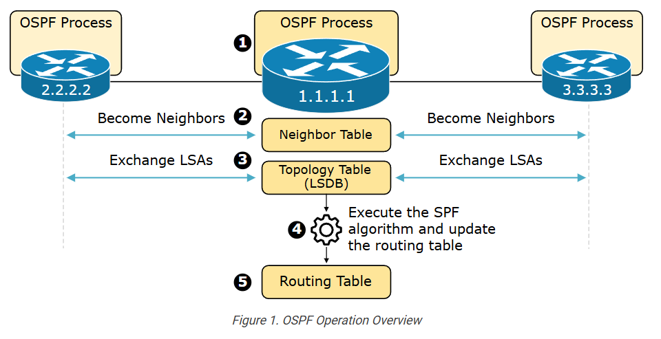
- Step 1. Enable the local OSPF process and choose RID: The first step in the OSPF operation is to enable the local process on each router. When the process initializes, it must allocate a unique Router ID (RID) to be able to send OSPF messages.
- Step 2. Establish neighbor adjacencies: Once the routing process is enabled on a router, it starts sending Hello messages on all OSPF-enabled links to determine whether neighbors are present on those segments. If other OSPF-enabled devices sit on the same segment, the router attempts to establish a neighbor adjacency with that device.
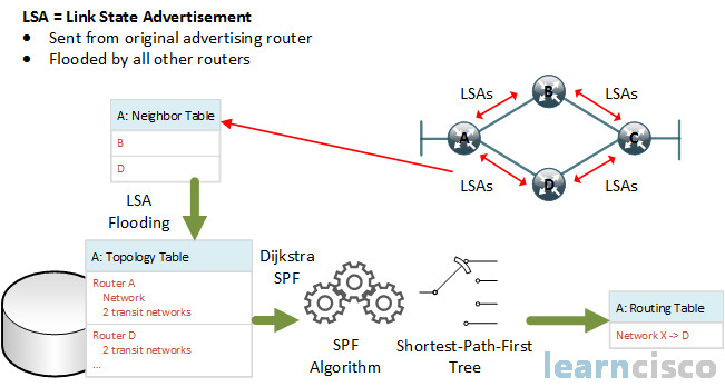
- Step 3. Exchange LSAs and build the topology table (the LSDB): After the router becomes adjacent to the neighboring OSPF devices, it starts exchanging LSAs. Link-state Advertisements (LSAs) contain each directly connected link’s cost and IP settings. Every router floods all LSAs to its neighbors until every device in the OSPF domain has all LSAs. This process is referred to as the LSA-flooding.
- The router builds the link-state database (LSDB) based on the received LSAs. The LSDB holds all the information about the network’s topology (hence, it is called the topology table). Because all LSAs are flooded to every router in the area, all routers in the same area have the same information in their LSDBs.
- Step 4. Execute the SPF algorithm: The LSDB serves as an input to the SPF algorithm. The algorithm calculates the best paths based on the advertised cost of each link and creates the SPF tree from the point of view of the local router.
- Step 5. Update the routing table with the best paths: Lastly, the router adds the best paths from the SPF tree into the routing table. The router then makes forwarding decisions based on the entries in the routing table.
Now, let’s walk through each step in more detail and discuss the most important aspects of the protocol.
Step 1. The OSPF Process
By default, the OSPF process is disabled on every Cisco IOS-XE device. It is enabled manually using the router ospf command via the CLI.
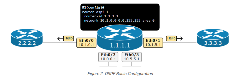
The diagram above serves as an example of the prerequisite involved in enabling the OSPF process on a device.
OSPF Versions
First, pay attention to the fact that the protocol has evolved through several versions:
- OSPFv1 was introduced in 1989. It was an experimental protocol and was never really used in production.
- OSPFv2 was introduced in 1991 as specified in RFC 1247, later updated by RFC 2328. It became the standard for IPv4 routing and is most widely adopted. In this course, we primarily discuss version 2.
- OSPFv3 was introduced in 2008 as specified in RFC 5340, later updated by RFC 5838. It has been designed to support IPv6 natively, but it also supports IPv4.
When you enable the OSPF process with ID 1 using the following command, you enable version 2.
R1(config)# router ospf 1
When you enable the process with ID 1 using the command below, you enable version 3.
R1(config)# router ospfv3 1
When you enable the process with ID 1 using the command below, you enable version 3.
Obviously, in our example shown in Figure 2, we enabled version 2 of the protocol.
The Process ID
When enabling the process on a router, you must specify a process ID. It is a locally significant number between 1 and 65535 (216-1) as you can see below.
					R1(config)# router ospf ?
  <1-65535>  Process ID
The OSPF process ID is only locally significant to the router. This means that different routers in the same OSPF network can use different process IDs without affecting OSPF operations.
The process ID allows multiple instances of OSPF to run on the same router. Each OSPF instance can be configured independently with its own set of parameters, areas, and interfaces.
The Router ID
The OSPF process requires a Router ID (RID) to initialize and be able to send messages. The RID is a unique 32-bit identifier. There are two options regarding the RID:
- You can directly configure the RID under the process. This is the recommended approach.
- You can leave the router to choose a RID automatically.
- The router tries to use the highest loopback IPv4 address.
- If loopback IP isn’t available, it tries to use the highest interface IPv4 address.
We are going to discuss the process of allocating an RID in greater detail later on. For now, let’s show an example of configuring a Router ID 1.1.1.1 on the router in the example.
					R1(config)# router ospf 1
R1(config-router)# router-id 1.1.1.1
R1(config-router)#
Remembering that the router ID must be unique within the entire network is very important.
The Network Command
The last prerequisite before the router can send messages and form adjacencies with other routers is to specify which interfaces will participate in the OSPF process and which area they will belong to. By default, none of the interfaces are included in the routing process. We include a range of interfaces using the network command with the following syntax.
					router ospf 1
 network <ip-address> <wildcard-mask> area <area-id>
The network command has two functions:
- It includes the interfaces that fall within the specified range in the OSPF process, meaning the router starts sending OSPF Hello packets to these interfaces.
- It advertises the prefix of the included interfaces within the OSPF domain.
The router checks each interface’s IP address against the specified IP address and wildcard mask in the network command. If an interface’s IP address falls within the specified range, the interface is included in the OSPF process for the given area.
Look at the example shown in Figure 2. Notice that the router has four interfaces – Eth0/0 through Eth0/3. However, only interfaces Eth0/0 (10.1.0.1) and Eth0/1 (10.1.5.1) are included in the OSPF process because their IP addresses match against the network command network 10.1.0.0 0.0.255.255 area 0. The IP addresses of the other two interfaces do not match against the network command and aren’t included. Hence, the router doesn’t send Hello messages over ports Eth0/2 and Eth0/3.
Step 2. The Neighbor Table
Step 1 is basically a prerequisite for every router in the network that wants to run OSPF. When two routers have successfully enabled the routing process, allocated RID, and have an OSPF-enabled interface on the same link, they can become neighbors.
Becoming OSPF Neighbors
The process of becoming OSPF neighbors can be broken down into two main phases, which we are going to discuss separately.
Becoming 2-Way Neighbors
Let’s look at the example shown in the diagram below, where two routers, R1 (1.1.1.1) and R2 (2.2.2.2), are directly connected via a link. Both routers have just been configured and the link between them has just been brought up.
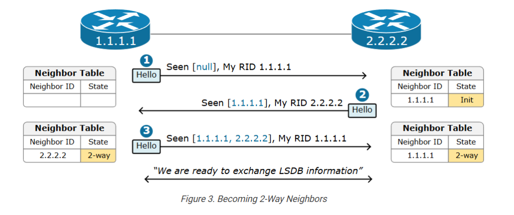
- Step 1. In the beginning, both devices have an empty neighbor table because none of them have received Hello packets. This is referred to as the Down state.
- Step 2. When R2 receives the Hello packet from R1 but does not see its own router ID in the Hello message, it transitions to the Init state. In this state, R2 records R1’s RID in its neighbor table and starts including R1’s RID in the Hello messages that it sends on this link.
- Step 3. When R1 receives the Hello packet from R2 and sees its own router ID in the Hello message, it transitions its neighbor state with R2 to the 2-Way state. This means that both routers recognize each other as neighbors. The process also takes place in the other direction until both become in a 2-way state.
Notice that there may be more routers sitting on the same link. In that case, every router includes all the RIDs it hears through received Hello packets in the Hello messages it sends.
Becoming Fully Adjacent
Once two routers become 2-way neighbors, they can start exchanging their Link-State Database information.
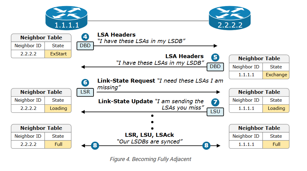
Steps 4 and 5. When R1 and R2 are in a 2-way state and decide to exchange their Link-State Databases (LSDBs), they do not simply send the entire LSDB to the remote neighbor. The entire database can be huge, and they may have almost identical LSDB. That’s why they first sent a summary list of all the LSAs they have in the LSDB. This is done using Database Description (DBD) packets.
Step 6. In the previous step, R2 sends a list of 50 LSAs that it has in the LSDB. R1 then queries its LSDB and finds that it misses only 5 LSAs from the list. Then R1 sends a Link-State Request (LSR) packet to request those 5 missing LSAs.
Step 7. R2 sends the full five LSAs that R1 requested in the previous step using a Link-State Update (LSU) packet. Notice that one LSU packet can hold multiple LSAs.
Step 8. In the end, the routers transition to Full state, meaning they have exchanged missing LSAs and now have identical LSDBs and views of the topology.
OSPF Packets
OSPF uses the following 5 packet types in the process of forming adjacencies and exchanging the LSDB database. The following table explains the function of each packet type. When you go through the table, go back and walk through the process of becoming neighbors again in the context of the packets used.
| OSPF Packet (encapsulated in IP with protocol number 89) | Description |
| Hello | Routers periodically send Hello packets to build and maintain OSPF neighbor adjacencies.
|
| Database Description (DBD) | When two routers become OSPF neighbors, they start exchanging their link-state information. The Database Description (DBD) packet is simply a summary of the router’s LSDB.
|
| Link-State Request (LSR) | If a router determines that it misses some LSAs, it sends a Link-State Request (LSR) packet to inform the neighbor to send the missing LSAs.
|
| Link-State Update (LSU) | There are several types of Link-State Update (LSU) packets, which are simply called LSAs.
|
| Link-State Acknowledgment (LSAck) | Link-State Acknowledgments (LSAcks) are sent to confirm the reception of an LSU. Routers must explicitly acknowledge each received LSA.
|
Now return to the process of establishing adjacency and look at in the context of the packet types that are used.
Step 3. The Topology Table (LSDB)
Once all routers in the network reach a full state, it means that all devices have the same Link-State Database (LSDB). This means that every device has the same view of the topology.
When a router wants to advertise a new link or change in the topology, it sends a link-state advertisement (inside an LSU), which is flooded to all devices in the OSPF domain so that each one has the same topology view. This process is referred to as LSA-flooding.
The LSA Flooding
The LSA flooding process ensures that all devices have a synchronized link-state database. The following diagram shows an example of the flooding process in a signal area network.
Upon receiving a new LSA, each device updates its LSDB database and runs the SPF algorithm to calculate the best paths to every network.
This process works well in small and medium networks with less than a hundred routers. However, it has some scaling limitations in large networks with hundreds of routers and thousands of links. Let’s walk through some of the sailing limitations, bearing in mind that the protocol is 30 years old.
- The LSDB becomes very large and requires a lot of RAM (back in the day, routers had a few MB of RAM)
- LSA flooding requires a lot of bandwidth (back in the day, links were 2Mbps and even less)
- The SPF algorithm requires a lot of CPU to run, translating to a lot of time to finish. (back in the day, devices had less powerful CPUs)
- Every event in the network (such as the interface going down -> up) forces every device to rerun the SPF algorithm.
Step 4. The SPF Algorithm
The LSA flooding process ensures that every device has the same LSDB database. However, it is very important to understand from the very beginning that the LSDB does not provide routing information that the router can directly add to its routing table. The LSDB describes the entire network topology – all routers and all links. It is like a map of the entire city. However, a map does not tell you the fastest route between point A and point B. The map shows you all available path and their properties (boulevard, highway, street, etc.) However, you must compare different routes yourself and consider each route’s capacity to select the fastest – highways are faster than city streets, which are faster than dirt roads, etc.
- LSDB is the map of the city. Every router is at a different place on the map.
- The SPF algorithm uses the map to find the fastest route from the local router to every remote destination.
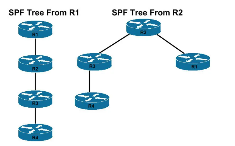
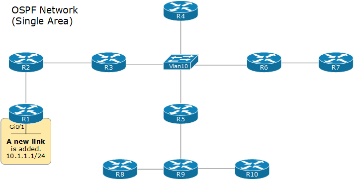
Let’s look at the diagram below, for example. Notice that each router has the same topology view of the network. However, every router must run the SPF algorithm to calculate the best route to every remote network from his local point of view. Because every router is at a different point in the topology. (every device is at a different place on the map)
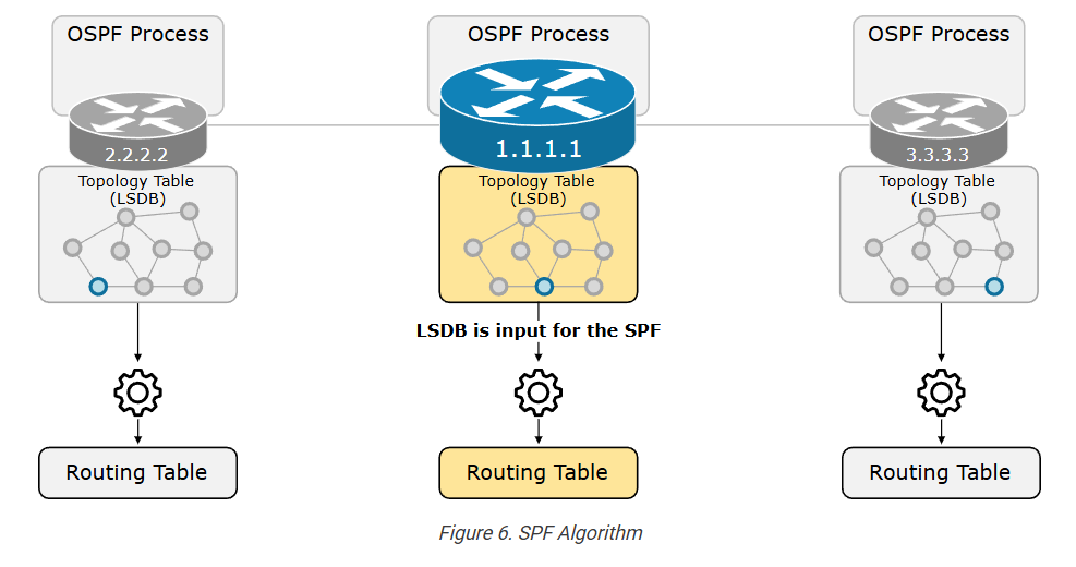
Every router must run the SPF algorithm on its own because the fastest route to network A could be different depending on each router’s specific location in the topology. For example, the fastest path from R1 to network A may be different from the fastest path from R2 to network A, and so on.
In that context, OSPF uses the Dijkstra Shortest Path First (SPF) algorithm to process the LSDB and build the best path to every known network from the local router’s point of view. The best routes the SPF algorithm calculates are then added to the routing table.
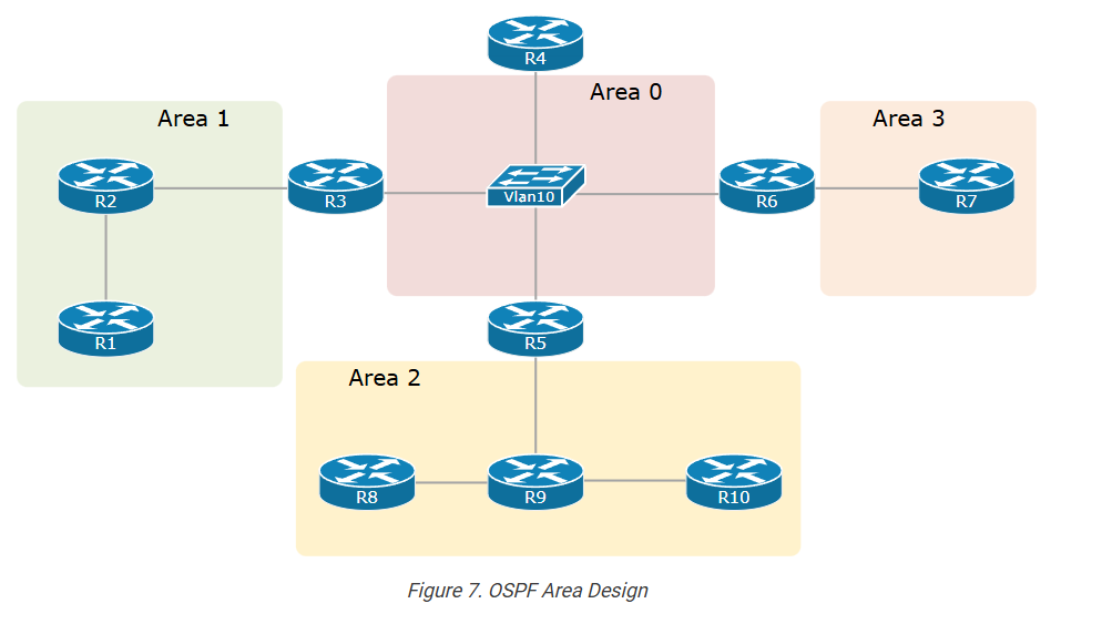
The Area concept
As we have already said, single-area OSPF design suffers when the network grows beyond 50+ routers. The solution to this scaling limitation is to break the network into several smaller network areas. For example, if a large single-area network is analogous to a large city, a network with multiple smaller areas is analogous to multiple smaller interconnected cities.
The area concept has multiple scaling benefits:
- The large LSDB is broken into smaller LSDBs per area.
- Each area has its own LSDB. For example, you only need to know the map of your city and the paths that lead to the other cities. You don’t need to know the paths within another city.
- Since the LSDB of each area is much smaller, the OSPF process requires less RAM and CPU and less time to run the SPF.
- Changes in one area require only the routers in that area to perform SPF calculations, significantly reducing the number of times SPF must run.
- The LSA flooding process happens only within the area, reducing the required bandwidth.
Key Takeaways
This lesson became larger than expected. We touched on the most important aspect of the link-state protocol. However, there is much more when you get into detail about how everything works and fits together. Anyway, let’s walk through the most important parts of the lesson.
The protocol works in five main steps:
- Step 1. Enable the local routing process and choose RID.
- Step 2. Establish neighbor adjacencies.
- Step 3. Exchange LSAs and build the topology table (the LSDB).
- Step 4. Execute the SPF algorithm.
- Step 5. Update the routing table with the best paths.
Neighborship States:
- Down State
- The initial state where no OSPF information has been exchanged between the routers.
- Init State
- A router sends a Hello packet from its interfaces to find OSPF neighbors.
- If a router receives a Hello packet that contains its router ID in the Neighbor field, it transitions to the 2-Way state.
- 2-Way State
- Both routers recognize each other as neighbors.
- The routers establish a full adjacency based on their roles (DR/BDR election).
- ExStart State
- The routers negotiate the master-slave relationship and the initial sequence number for the DBD (Database Description) packets.
- The router with the higher router ID becomes the master.
- Exchange State
- The routers exchange DBD packets, which contain summaries of their link-state databases.
- These summaries include LSA (Link-State Advertisement) headers, which help identify missing or outdated LSAs.
- Loading State
- The routers send LSRs (Link State Requests) for any LSAs they need based on the summaries received in the Exchange state.
- The neighbors respond with LSU (Link State Update) packets containing the requested LSAs.
- Full State
- Both routers have the same link-state database.
- They have completed the exchange of LSAs and are fully adjacent.
- OSPF routing can now occur based on the complete and synchronized link-state database.
OSPF Packets:
- Hello
- Periodically sent to 224.0.0.5.
- Discover other OSPF routers onto the same segment/link.
- Includes information about the sending router – such as RID, Area ID and Authentication Type.
- Determines whether adjacency will form.
- Database Descriptor (DBD)
- A summary of LSA’s in the router’s LSDB.
- It avoids sending the full LSDB data unnecessarily.
- Link-State Request (LSR)
- Sent to request a list of full LSAs.
- Link-State Update (LSU)
- Includes requested LSAs.
- Link-State Acknowledgment (LSAck)
- Sent to confirm the reception of LSU.
OSPF Packet Type Details
1. Hello Packet (Discover Neighbors)
Purpose: To find and maintain neighbor routers.
- Routers send Hello packets periodically on a network.
- When another router receives the Hello packet, it knows a neighbor exists.
- If the parameters match (area ID, subnet, timers, etc.), they become neighbors.
Functions:
- Discover neighboring routers
- Check if neighbors are still alive
- Elect Designated Router (DR) and Backup Designated Router (BDR)
Example:
Router A sends Hello → Router B replies → Neighbor relationship established.
2. DBD – Database Description Packet
Purpose: To summarize the routing database between routers.
- After routers become neighbors, they exchange DBD packets.
- These packets contain summaries of the Link-State Database (LSDB).
- This helps routers compare their databases.
Key idea:
Routers say:
“Here is the list of routes I know. Do you have the same?”
3. LSR – Link State Request
Purpose: To request specific routing information.
- If a router sees missing or outdated entries in the database summary, it sends an LSR.
- This packet asks for the complete information about a specific route.
Example:
Router A: “I don’t have this route. Please send full details.”
4. LSU – Link State Update
Purpose: To send the requested or updated routing information.
- The router responds to LSR with LSU packets.
- LSU contains Link State Advertisements (LSAs).
- LSAs describe the network topology.
Example:
Router B sends LSU → full route information to Router A.
5. LSAck – Link State Acknowledgement
Purpose: To confirm that LSU was received successfully.
- When a router receives an LSU, it sends LSAck.
- This ensures reliable delivery of routing information.
Example:
Router A: “I received the update successfully.”
Simple Communication Flow in OSPF
- Hello → Discover neighbors
- DBD → Exchange database summaries
- LSR → Request missing information
- LSU → Send full routing information
- LSAck → Acknowledge receipt
Hello Packet Contains
In Open Shortest Path First (OSPF), the Hello Packet contains several fields that help routers discover neighbors and build adjacency.
1. Network Mask
The Network Mask field shows the subnet mask of the interface sending the Hello packet. Neighbor routers must have the same subnet mask to form an OSPF relationship. If the subnet mask does not match, the routers will ignore the Hello packet and no neighbor adjacency will be formed.
2. Hello Interval
The Hello Interval defines how often a router sends Hello packets to neighbors. In most broadcast and point-to-point networks, the default Hello interval is 10 seconds. All routers in the same OSPF network segment must have the same Hello interval.
3. Dead Interval
The Dead Interval specifies how long a router waits to receive a Hello packet before declaring a neighbor router down. Normally it is four times the Hello interval. For example, if the Hello interval is 10 seconds, the Dead interval is usually 40 seconds.
4. Router ID
The Router ID is a unique 32-bit identifier used to identify each OSPF router in the network. It is usually written in an IP address format like 1.1.1.1. This ID helps routers recognize which device sent the Hello packet.
5. Area ID
The Area ID identifies the OSPF area to which the router belongs. For routers to become neighbors, they must be in the same OSPF area. The most important area is Area 0, known as the backbone area.
6. Authentication
The Authentication field is used to secure OSPF communication. It ensures that only authorized routers participate in the routing process. Authentication types include no authentication, simple password authentication, and MD5 authentication.
7. Router Priority
The Router Priority value is used for Designated Router (DR) and Backup Designated Router (BDR) election in broadcast networks. A router with a higher priority has a greater chance of becoming the DR. The default priority value is usually 1.
8. Designated Router (DR) Address
This field shows the IP address of the Designated Router for the network segment. The DR is responsible for managing routing updates between OSPF routers in broadcast networks.
9. Backup Designated Router (BDR) Address
This field contains the IP address of the Backup Designated Router. The BDR takes over the role of DR if the DR fails.
10. Neighbor Router IDs
The Neighbor field lists the Router IDs of neighboring routers from which Hello packets have already been received. When a router sees its own Router ID in this list, it confirms a two-way communication state with the neighbor.


Parameters Must Match OSPF Neighbor Adjacency
For routers to form adjacency in Open Shortest Path First (OSPF), several parameters must match between the routers. If these parameters are different, OSPF neighbor adjacency will not form.
1. Area ID
Both routers must be in the same OSPF area.
Example:
Router A → Area 0
Router B → Area 0
If different areas → adjacency will not form.
2. Hello Interval
The Hello timer must be the same on both routers.
Example:
Router A → 10 seconds
Router B → 10 seconds
3. Dead Interval
The Dead timer must also match.
Example:
Router A → 40 seconds
Router B → 40 seconds
4. Network Mask
The subnet mask of the interface must be identical.
Example:
Router A → 255.255.255.0
Router B → 255.255.255.0
5. Authentication
If authentication is configured, both routers must use the same authentication type and password.
Example:
MD5 key must match.
6. Stub Area Flag
If the area is configured as a stub area, both routers must have the same stub configuration.
7. Network Type (Important)
The OSPF network type should match.
Example:
- Broadcast
- Point-to-Point
- NBMA
8. MTU (in some cases)
If the MTU size is different, adjacency may get stuck in EXSTART/EXCHANGE state.
Summary (Most Important Matching Parameters)
- Area ID
- Hello Interval
- Dead Interval
- Subnet Mask
- Authentication
- Stub Area flag
- Network Type
- MTU (recommended to match)
OSPF State
7 States Of OSPF
- Down: no OSPF neighbors have been detected at this moment.
- Init: Hello packet received.
- Two-way: own router ID found in received hello packet.
- Exstart: master and slave roles determined.
- Exchange: database description packets (DBD) are sent.
- Loading: exchange of LSRs (Link state request) and LSUs (Link state update) packets.
- Full: OSPF routers now have an adjacency


What is SPF (Algorithm Shortest Path First)
SPF (Shortest Path First) is the algorithm used in Open Shortest Path First (OSPF) routing protocol to determine the best and shortest path from one router to all other networks in an OSPF area. The SPF algorithm analyzes the complete network topology and calculates the lowest-cost routes. It is based on Dijkstra’s Algorithm, which is designed to find the shortest path between nodes in a graph.
In OSPF, every router builds a Link-State Database (LSDB) that contains information about all routers and links in the network. This database is created using Link-State Advertisements (LSAs) that routers exchange with each other. Because all routers share the same LSDB, each router has a full map of the network topology. After building this map, the router runs the SPF algorithm to calculate the shortest path to every destination network.
The SPF algorithm works by starting from the router itself (called the root node) and calculating the cost of reaching each neighboring router. The algorithm then gradually examines all possible paths through the network and chooses the path with the lowest total cost. OSPF cost is usually based on bandwidth, meaning higher bandwidth links typically have lower cost values. The path with the smallest cumulative cost becomes the best route and is installed in the router’s routing table.
SPF calculation is not performed continuously; it runs only when there is a change in the network topology. Such changes may include a router going down, a new router joining the network, a link failure, or receiving a new link-state update. When such an event occurs, routers flood updated LSAs throughout the OSPF area. After updating the LSDB, each router runs the SPF algorithm again to recompute the best routes.
One important advantage of SPF in OSPF is that it provides fast and accurate routing decisions because every router independently calculates routes using the same topology information. This makes OSPF more efficient and scalable compared to older distance-vector protocols. However, SPF calculations can consume CPU resources in very large networks, so OSPF uses optimization techniques such as incremental SPF and timers to reduce unnecessary recalculations.
In summary, SPF is the core process that allows OSPF routers to analyze the network topology and determine the shortest and most efficient paths for data transmission. By using Dijkstra’s algorithm and link-state information, OSPF ensures reliable, loop-free, and optimized routing across complex networks.
SPF in OSPF
SPF stands for Shortest Path First. It is the algorithm used by Open Shortest Path First (OSPF) to find the best (shortest) path to reach a network.
SPF is based on the Dijkstra’s Algorithm.
What SPF Does
SPF calculates the shortest path between routers using the information in the Link-State Database (LSDB).
Each router:
- Collects network information from other routers.
- Builds a network topology map.
- Runs the SPF algorithm.
- Finds the lowest-cost path to each network.
- Adds the best path to the routing table.
When SPF Runs
SPF calculation runs when:
- A new router joins the network
- A link goes down
- A link state update (LSU) is received
- The network topology changes
Simple Definition (for exams)
SPF (Shortest Path First) is the algorithm used by OSPF to calculate the shortest path to all networks based on link cost.