What Is OSPF
History Of OSPF
Open Shortest Path First (OSPF) is a link-state routing protocol used in IP networks to find the shortest path for data packets between routers. It is widely used in enterprise and service provider networks because it converges quickly and supports large, complex network designs.
History of OSPF
The development of OSPF started in the 1980s when older routing protocols such as Routing Information Protocol (RIP) were commonly used. RIP had many limitations, such as a maximum hop count of 15, slow convergence, and poor scalability for large networks. Because of these limitations, network engineers needed a more advanced routing protocol for growing networks.
To solve these problems, the Internet Engineering Task Force (IETF) began developing OSPF as an open standard routing protocol. The goal was to create a protocol that could support large enterprise networks, faster convergence, and better routing decisions compared to RIP.
The first official version, OSPF Version 1, was published in 1989 in RFC 1131, but it was mostly experimental. Later, a more stable version called OSPF Version 2 was released in 1991 (RFC 1247) and became widely used for IPv4 routing in enterprise networks.
As networks evolved to support IPv6, a new version called OSPF Version 3 was introduced in 2008 (RFC 5340). OSPFv3 was designed specifically to support IPv6 routing and modern network requirements.
Summary
In simple terms, OSPF was developed to replace older routing protocols like RIP and provide faster, more scalable, and efficient routing. Today, OSPF is one of the most widely used Interior Gateway Protocols (IGPs) in enterprise and service provider networks.
OSPF at a high level
Let’s start at a higher level, as simple as possible. OSPF is a link-state routing protocol that uses a mathematical algorithm to determine the best path to every IP destination in the network. For example, if you have a network with a hundred routers running OSPF, each router knows how to reach every destination in the network via the most optimal path.
The OSPF Network
Suppose we have a large enterprise network like the one shown in the diagram below. There are many different network paths between every two sites. Network administrators have two choices:
- They can manually configure each router in the network with the best path to each destination and then reconfigure it again on link failure.
- Or they can use a dynamic routing protocol such as OSPF that automatically calculates the best paths and reacts to link failures and topology changes.
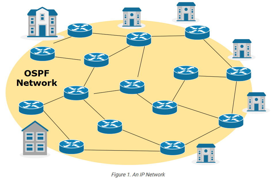
Of course, every organization uses a dynamic routing protocol, and OSPF is among the most popular. It has been around for 30+ years. It has been widely adopted worldwide in enterprise, data center, and service provider networks.
However, for someone new to IP networking, this creates a false impression that OSPF is somehow a centralized network function. The reality is that each router in the network runs an independent local instance of the OSPF protocol.
However, using OSPF messages, each router advertises practically every detail about every connected link. This results in all routers collectively accumulating information about every device and network in the environment. Subsequently, every router knows how to reach every IP destination via the optimal network path.
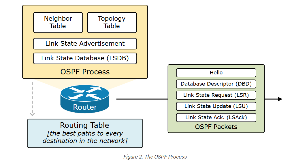
The OSPF Process
From a single router perspective, OSPF is a process that runs on the device alongside all other processes. It uses a set of tables, databases, and messages to exchange information with other routers. The ultimate goal of the routing process is to update the device’s routing table with the best paths, as shown in Figure 2.
By default, the OSPF process is disabled on all Cisco IOS and IOS-XE devices. We start the process using a global configuration command and assigning a process ID. The process ID does not need to match all routers within the network. It is a local identifier used to identify a specific instance of the OSPF routing process running on that router. It is purely local and has no significance outside the router. For example:
					Router# conf t
Enter configuration commands, one per line.  End with CNTL/Z.
Router(config)# router ospf ?
  <1-65535>  Process ID
Router(config)# router ospf 1
Router(config-router)# end
Router#
Once we enable the OSPF process, the device first tries to assign a router ID. If it does not succeed, the process cannot start, as you can see in the log below.
					*Jul  9 14:47:06.725: %OSPF-4-NORTRID:
OSPF process 1 failed to allocate unique router-id and cannot start
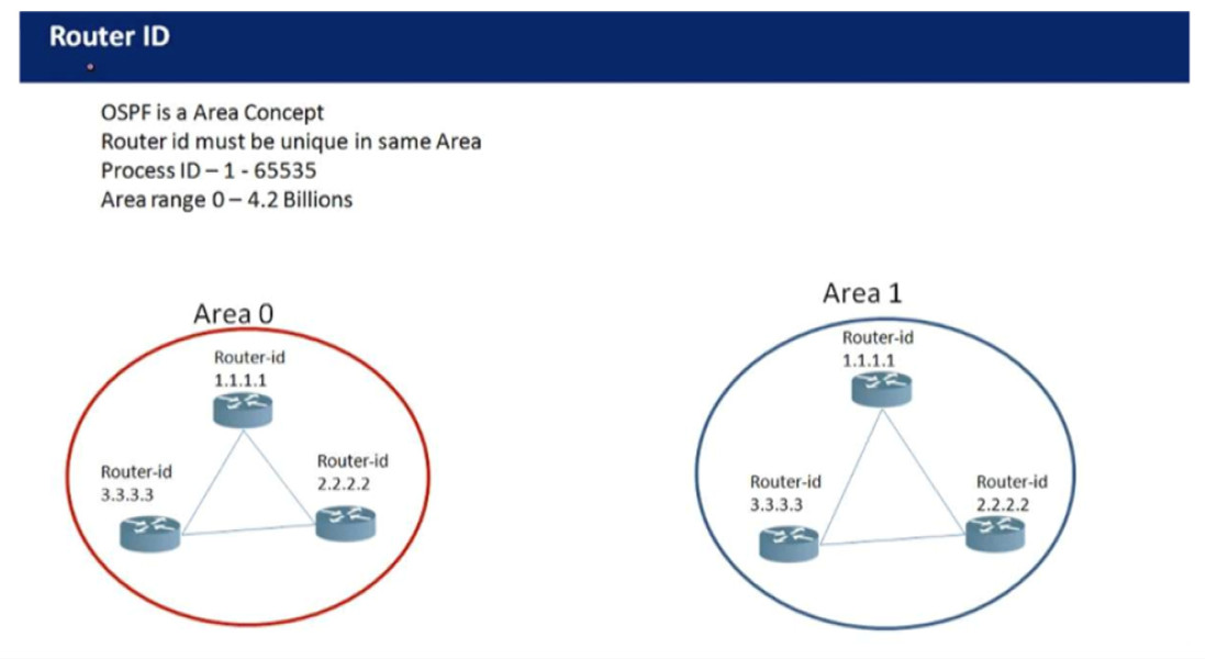
The Router ID
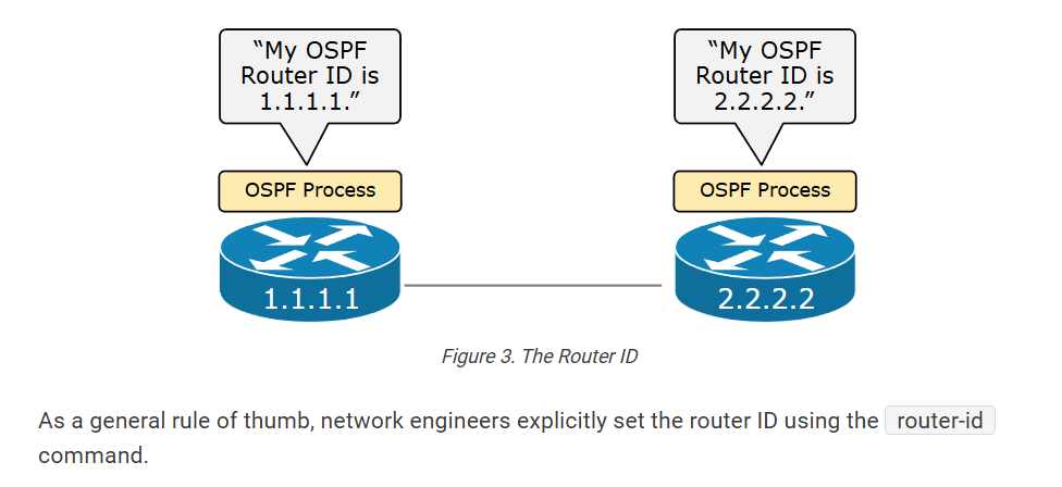
When it initializes, the OSPF process tries to allocate a unique 32-bit identifier called the Router ID (RID). The process cannot generate and send messages without an RID.
Each router uses the following steps when trying to assign the RID:
- Step 1. First, the router checks if a router ID is explicitly configured via the router-id command under the OSPF process.
- Step 2. If no ID is explicitly provided, the router tries to use the highest loopback IP address, which is not in the admin shutdown state.
- Step 3. If the router still cannot assign RID at step 2, it tries to use the highest non-loopback IP address.
Becoming Neighbors
Once the OSPF process on a router has successfully chosen a Router ID, it starts sending Hello messages on all OSPF-enabled interfaces.
When two routers sit on the same VLAN, Serial, or WAN link, they hear each other’s Hello messages and become neighbors, as shown below.
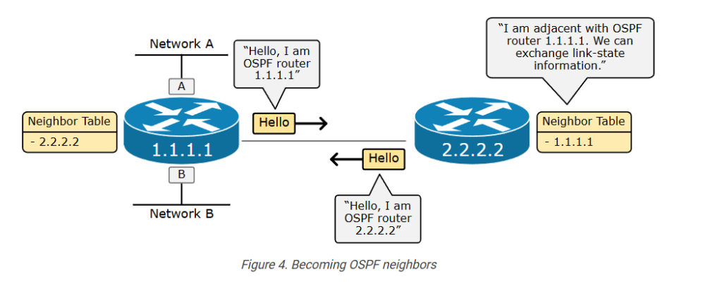
The neighbor model has two primary functions:
- It allows routers to dynamically discover new OSPF routers on a shared segment without requiring manual configuration from a network administrator.
- It allows the routers to exchange their link-state network knowledge.
The following output shows how we check the neighbors of a router.
					R1# sh ip ospf neighbor
Neighbor ID   Pri   State     Dead Time   Address    Interface
2.2.2.2         1   FULL/DR   00:00:38    10.1.1.2   Ethernet0/0
Exchanging Database Information
Once two devices become neighbors, the next step is to exchange their link-state database information. Let’s break down what link-state means:
- A link is simply a router interface. Look at the diagram below, for example. Interface A is a link. Interface B is another link. Interface C is another, and so on.
- The link state describes the interface’s properties, such as its IP address and mask, interface type, relationship with neighboring routers, and so on.
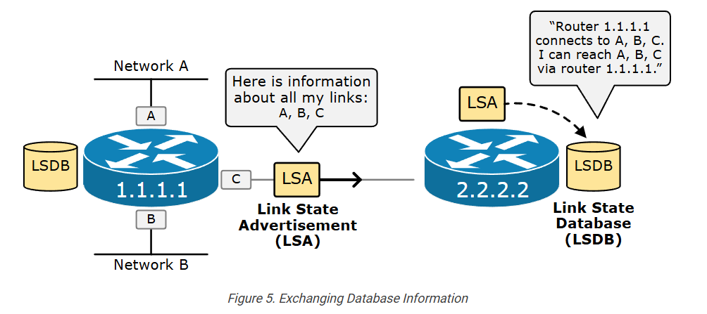
For example, router 1.1.1.1 has three links: A, B, and C. Using a Link-State Advertisement (LSA), the router shares the link-state information about A, B, and C with its neighboring router 2.2.2.2.
LSA flooding
If we look at the database exchange process on a larger scale, we can see how the link-state advertisement process works. Suppose we have just added a new link on router 1.1.1.1, as shown in the diagram below. To ensure that every router knows that a new link with IP 10.1.1.1 that connects to 10.1.1.0/24 exists, router 1.1.1.1 sends a new LSA update to all neighbors. Each router then resends the LSA to all other neighbors until every router receives a copy of the LSA. This process is called the LSA flooding.
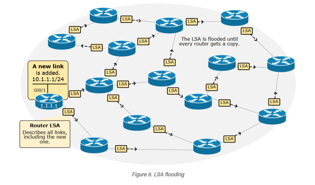
Of course, there is a loop prevention mechanism that ensures an LSA update does not circle around indefinitely. However, a more important question is—how does this LSA flooding process scale? What if we have a network with 250 routers? Every single LSA update must be flooded to all 250 routers, which means, in practice, that every link-state change (for example, a link goes down) creates a flood of LSA across the entire network.
The LSDB (Link-State Database)
Every router stores the LSAs it receives into a database called the Link-State Database (LSDB). Since the LSA flooding ensures that every router receives a copy of every LSA, each router in the OSPF network maintains an identical LSDB and has a consistent view of the network.
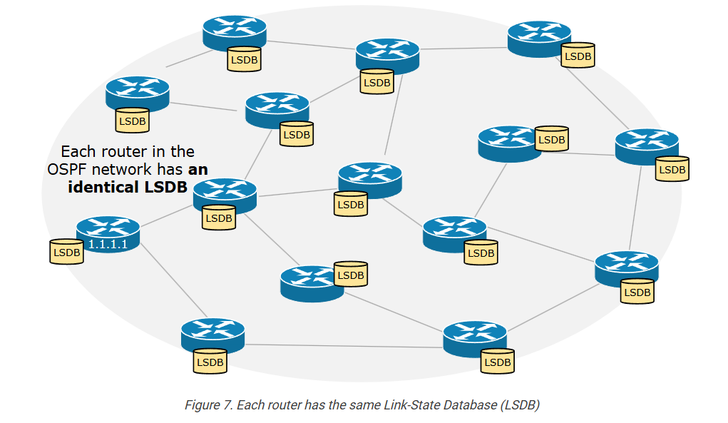
When a router receives a new LSA, it updates its link-state database and forwards the LSA to its neighbors, ensuring all routers have the same LSDB.
The SPF Algorithm
Another important aspect of OSPF is that LSAs do not contain routing information that the router can directly add to its routing table. An individual LSA is simply one piece of link-state information. All received LSAs make up the Link-state database (LSDB), which contains all information about the entire network. However, the LSDB does not provide routing information. It is a collection of all received LSAs.
The OSPF’s mathematical algorithm, SPF, uses the information in the link-state database as an input to calculate the shortest paths that the router must add to its routing table, as shown in the diagram below.
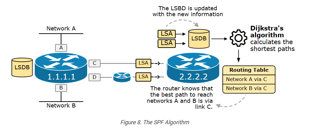
The SPF uses Dijkstra’s algorithm for finding the shortest path between nodes.
Here, it is important to understand that even though the LSDB is the same on all devices in the topology, the SPF algorithm, also known as Dijkstra’s algorithm, uses the LSDB to calculate the shortest path tree for the local router. This tree represents the best paths to all destinations in the OSPF network from the local router’s perspective. For example, every device has different best paths to network A.
Link Cost
One of the link-state properties of a link is called “cost.” It is a numerical value assigned to each link between routers. This cost represents the “expense” or “distance” of sending packets over that link.
The SPF (Shortest Path First) algorithm uses the link cost to calculate the network’s shortest and most efficient path. Lower cost values indicate preferred links, leading to optimal routing decisions.
OSPF commonly uses the link’s outgoing bandwidth to determine its cost. Higher bandwidth links typically have lower costs, making them more attractive for routing decisions. The default formula used by many OSPF implementations for calculating cost is:

The Reference Bandwidth is a fixed value (usually 100 Mbps) that can be adjusted based on network requirements. The Link Bandwidth is the actual bandwidth of the link. For example, the following Ethernet interface has 10Mbps bandwidth, which translates to cost 100/10 = cost 10. Another example is a 100Mbps interface with a cost of 100/100 = 1.
					R1# sh ip ospf interface
Ethernet0/0 is up, line protocol is up
  Internet Address 10.1.1.1/24, Interface ID 2, Area 0
  Attached via Network Statement
  Process ID 1, Router ID 1.1.1.1, Network Type BROADCAST, Cost: 10
  Topology-MTID    Cost    Disabled    Shutdown      Topology Name
        0           10        no          no            Base
  Transmit Delay is 1 sec, State BDR, Priority 1
  Designated Router (ID) 2.2.2.2, Interface address 10.1.1.2
  Backup Designated router (ID) 1.1.1.1, Interface address 10.1.1.1
  Timer intervals configured, Hello 10, Dead 40, Wait 40, Retransmit 5
    oob-resync timeout 40
    Hello due in 00:00:05
  Supports Link-local Signaling (LLS)
  Cisco NSF helper support enabled
  IETF NSF helper support enabled
  Can be protected by per-prefix Loop-Free FastReroute
  Can be used for per-prefix Loop-Free FastReroute repair paths
  Not Protected by per-prefix TI-LFA
  Index 1/1/1, flood queue length 0
  Next 0x0(0)/0x0(0)/0x0(0)
  Last flood scan length is 1, maximum is 1
  Last flood scan time is 0 msec, maximum is 1 msec
  Neighbor Count is 1, Adjacent neighbor count is 1
    Adjacent with neighbor 2.2.2.2  (Designated Router)
  Suppress hello for 0 neighbor(s)
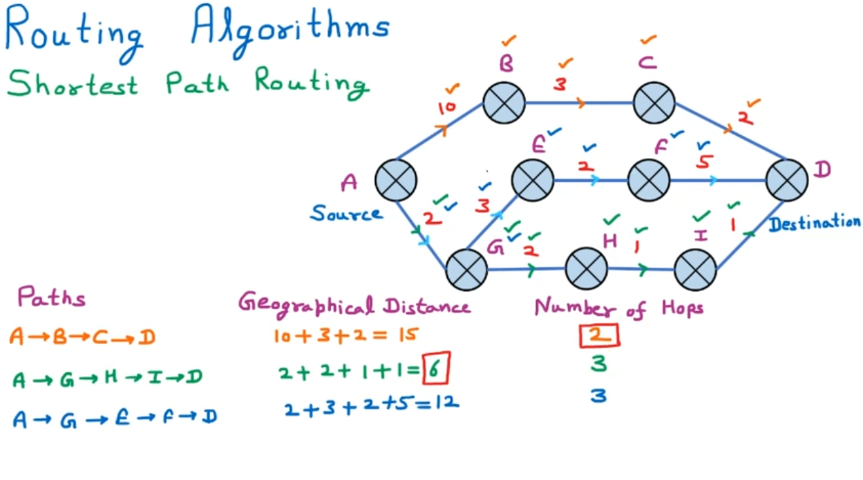
Let’s look at the following diagram as an example of how the cost works.
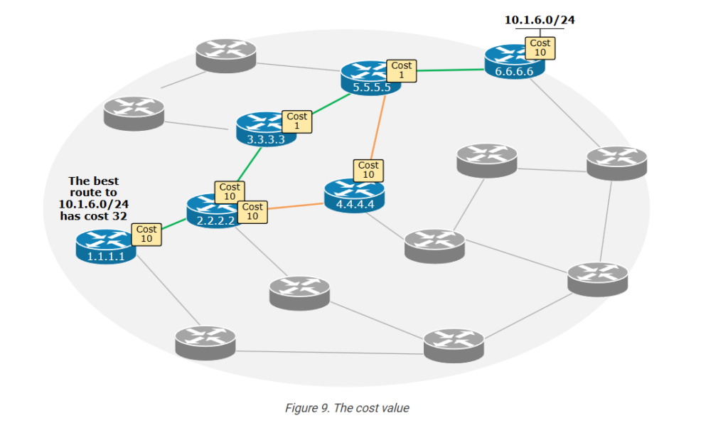
Router 1.1.1.1 has multiple paths to reach subnet 10.1.6.0/24. However, the diagram shows the two paths with lower costs. Let’s compare them and see why the one in green is the best.
					1.1.1.1 - 2.2.2.2 - 3.3.3.3 - 5.5.5.5 - 6.6.6.6	10+10+1+1+10 = 32 (best)
1.1.1.1 - 2.2.2.2 - 3.3.3.3 - 4.4.4.4 - 6.6.6.6	10+10+10+1+10 = 41
The SPF algorithm uses the link costs from the LSDB to build a shortest path tree. It adds up the costs of the links along potential paths and selects the path with the lowest total cost. The following output shows an example of the best route to 10.1.6.0/24 from the point of view of R1. Notice that the route metric (highlighted in yellow) is 32, which is the total cost of reaching the destination.
					R1# sh ip route
Codes: L - local, C - connected, S - static, R - RIP, M - mobile, B - BGP
       D - EIGRP, EX - EIGRP external, O - OSPF, IA - OSPF inter area
       N1 - OSPF NSSA external type 1, N2 - OSPF NSSA external type 2
       E1 - OSPF external type 1, E2 - OSPF external type 2, m - OMP
       n - NAT, Ni - NAT inside, No - NAT outside, Nd - NAT DIA
       i - IS-IS, su - IS-IS summary, L1 - IS-IS level-1, L2 - IS-IS level-2
       ia - IS-IS inter area, * - candidate default, U - per-user static route
       H - NHRP, G - NHRP registered, g - NHRP registration summary
       o - ODR, P - periodic downloaded static route, l - LISP
       a - application route
       + - replicated route, % - next hop override, p - overrides from PfR
       & - replicated local route overrides by connected
Gateway of last resort is not set
      10.0.0.0/8 is variably subnetted, 3 subnets, 2 masks
C        10.1.1.0/24 is directly connected, Ethernet0/0
L        10.1.1.1/32 is directly connected, Ethernet0/0
O        10.1.6.0/24 [110/32] via 10.1.1.2, 00:00:57, Ethernet0/0
Now, having seen how the protocol works, let’s shift the focus to the scaling side of things. What if the network grows to hundreds or thousands of devices?
Scaling the LSA-flooding process
We have seen how the LSA flooding process works to ensure that each device in the network maintains the same link-state database (LSDB). However, this LSA flooding process imposes a few scaling limitations:
- Every LSA update must be flooded to all devices. What if the network has 1,000+ routers and 10,000+ links? Imagine what the flooding process will look like.
- If a network has 10,000+ links, thousands of LSA updates will occur. These LSAs must be stored in the link-state database (LSDB), which requires a lot of RAM memory. Routers’ RAM is expensive – especially back in the old days when routers had a few MB of memory (keeping in mind that the protocol is 30+ years old).
- Each new LSA triggers an update of the LSDB database, which initiates a new run of the SPF algorithm, which requires a lot of processing power.
- The SPF algorithm takes more time to run when the link-state database is larger, which makes reacting to topology changes slower.
In short, the protocol requires more resources when scaling. More routers equal more CPU and RAM and slower convergence time.
To account for these scaling limitations, the protocol incorporates the concept of areas.
Areas
To scale, OSPF implements the area concept. An area is a segment of the network where routers exchange routing information. It helps in scaling large networks by dividing them into smaller sections, reducing the amount of routing information each device must process and store.
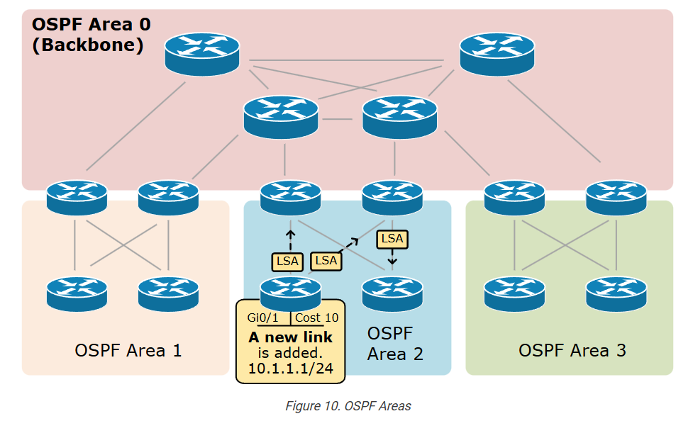
The area concept brings the following efficiency improvements:
- Link state advertisements (LSA) are only flooded into the area. For example, when we add a new link, as shown in the diagram above, the LSA update is only sent to the routers in Area 2. Compare this process to the one shown in Figure 6 above.
- Each area has its own link-state database (LSDB) – Since LSAs are only flooded within an area, only the devices within that area maintain the same LSDB, which makes the database smaller. This is a massive optimization from a performance point of view (required CPU and RAM memory).
- Changes in one area do not affect the other areas, which improves the convergence time. The devices in Area 1 do not need to run the SPF algorithm when a new link is added in Area 2, which optimizes the CPU usage.
Areas are a big concept that we discuss in great detail later in the course. However, here, we simply want to emphasize why they are required and important.
Key Takeaways
- OSPF is a link-state dynamic routing protocol. Its primary function is to calculate the best path to each IP destination in the network.
- A link is simply a router interface.
- The link state describes the interface’s properties, such as its IP address and Subnet Mask, interface type, and relationship with neighboring routers.
- Each router in the network runs an independent local instance of the OSPF protocol.
- To start, the process needs a unique 32-bit Router ID.
- Multiple routers become neighbors when they sit on the same VLAN or data link.
- The function of the neighboring process is to dynamically discover new OSPF routers without requiring manual reconfiguration.
- Another function of the neighboring process is allowing the routers to exchange link-state information.
- OSPF uses an LSA flooding mechanism to distribute each link-state advertisement to every router in the network.
- The LSA a router receives is stored in a database called the Link-State Database (LSDB).
- When a router receives an LSA, it updates its LSDB and forwards the LSA to its neighbors, ensuring that all routers maintain the same LSDB.
- The LSDB is an input to the Dijkstra algorithm that calculates each network node’s shortest paths.
- The concept of areas allows the protocol to scale efficiently.
OSPF – Open Shortest Path First
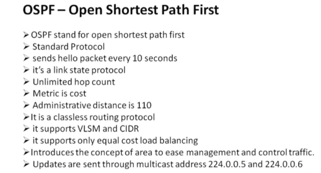
- OSPF stand for Open Shortest path first
- Standard protocol
- It’s a link state protocol
- It uses SPF (shortest path first) or dijkistra algorithm
- Unlimited hop count
- Metric is cost (cost=10 ^8/B.W.)
- Administrative distance is 110
- It is a classless routing protocol
- It supports VLSM and CIDR
- It supports only equal cost load balancing
- Introduces the concept of Area’s to ease management and control traffic
- Provides hierarchical network design with multiple different areas
- Must have one area called as area 0
- All the areas must connect to area 0
- Scales better than Distance Vector Routing protocols.
- Supports Authentication
- Updates are sent through multicast address 224.0.0.5
- Faster convergence.
- Sends Hello packet every 10 seconds
- Trigger/Incremental updates
- Router’s send only changes in updates and not the entire routing tables in periodicupdates
The OSPF protocol supports a couple of cool features such as
- CIDR
- Subdividing an Autonomous System into areas
- Equal Load balancing
- Fast convergence
- Multicast updates
- Authentication
- Large networks (significant number of routers)
- Open standard (implemented by different router vendors)
- Loop free routing protocol
- Route summarization
Now, let’s explain some of those features.
Open standard protocol: OSPF is not vendor proprietary, and it is deployed by lots of network device vendors such as Cisco, Juniper, Sophos, HP, Dell, Huawei, MikroTik, and more.
OSPF Packets Types
- Hello: neighbor discovery, build neighbor adjacencies, and maintain them.
- DBD: This packet is used to check if the LSDB between the two routers is the same. The DBD is a summary of the LSDB.
- LSR: Requests specific link-state records from an OSPF neighbor.
- LSU: Sends specific link-state records that were requested. This packet is like an envelope with multiple LSAs in it.
- LSAck: OSPF is a reliable protocol, so we have a packet to acknowledge the others.
Full From
- Hello (discover neighbors)
- DBD (database description)
- LSR (link state request)
- LSU (link state update)
- LS ack (link state acknowledge)
Slide Of OSPF


Advantages And Disadvantages in OSPF
Advantages of OSPF
1. Fast Convergence
One major advantage of OSPF is its fast convergence time. When a network change occurs, such as a link failure, OSPF quickly recalculates the best path and updates the routing tables of all routers. This helps reduce network downtime and ensures that data packets reach their destination quickly.
2. Supports Large Networks
OSPF is designed for large and complex enterprise networks. It uses a hierarchical design with areas, which helps divide the network into smaller segments. This structure reduces routing table size and improves network performance in large organizations.
3. Uses Cost-Based Routing
OSPF selects the best path based on link cost, which usually depends on bandwidth. This means the protocol chooses faster and more efficient paths instead of just counting hops like Routing Information Protocol. Because of this, network traffic is routed more efficiently.
4. Supports Load Balancing
OSPF allows equal-cost load balancing, which means if there are multiple paths with the same cost, it can distribute traffic across them. This improves network performance and prevents a single link from becoming overloaded.
5. Open Standard Protocol
OSPF is an open standard developed by the Internet Engineering Task Force. Because of this, it can work with routers from different vendors such as Cisco, Juniper, and others.
Disadvantages of OSPF
1. Complex Configuration
OSPF configuration is more complex compared to simpler routing protocols like RIP. Network administrators must understand areas, link-state databases, and routing calculations, which can make implementation more difficult.
2. High Resource Usage
OSPF requires more CPU power and memory on routers because it maintains a full link-state database and runs complex algorithms to calculate the shortest path. This can increase the load on network devices.
3. Difficult Troubleshooting
Because OSPF has many components such as areas, neighbor relationships, and LSAs, troubleshooting problems can be more complicated compared to simpler routing protocols.
4. More Initial Setup Time
Designing an OSPF network requires proper planning, especially when using multiple areas. If the network design is not correct, it can cause routing inefficiencies or instability.
In simple terms: OSPF is a powerful and fast routing protocol for large networks, but it requires more configuration knowledge and router resources compared to simpler protocols.
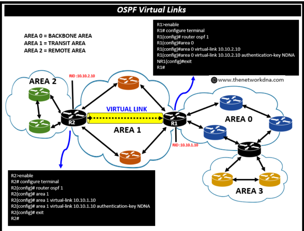
What is OSPF Area 0
1. Definition of Area 0
Area 0 is the backbone area of OSPF (Open Shortest Path First). It is the central area through which all other OSPF areas must communicate. It is also called the OSPF backbone.
2. Importance of Area 0
Area 0 is the most important part of an OSPF network because all inter-area communication must pass through it. If Area 0 is not properly configured, different areas cannot exchange routing information.
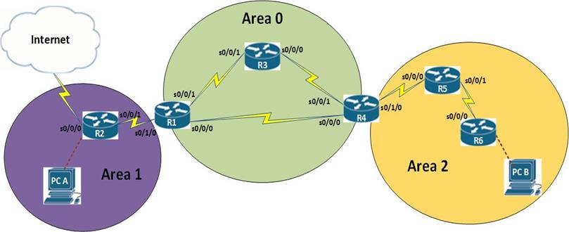
3. Role in OSPF Design
In a multi-area OSPF design, all other areas (like Area 1, Area 2, etc.) must be connected to Area 0 either directly or through a virtual link. This ensures a proper hierarchical structure and efficient routing.
4. Backbone Function
Area 0 acts as a central transit area. It carries routing information between different areas using ABR (Area Border Routers). Without Area 0, OSPF cannot function properly in multi-area networks.
5. LSA Flow in Area 0
Area 0 handles important LSAs such as:
- Type 3 (Summary LSA)
- Type 4 (ASBR Summary LSA)
- Type 5 (External LSA)
These LSAs help distribute routing information between areas.
6. Connectivity Rule (Important Exam Point)
All OSPF areas must connect to Area 0. If a direct connection is not possible, OSPF uses a virtual link to logically connect the area to Area 0.
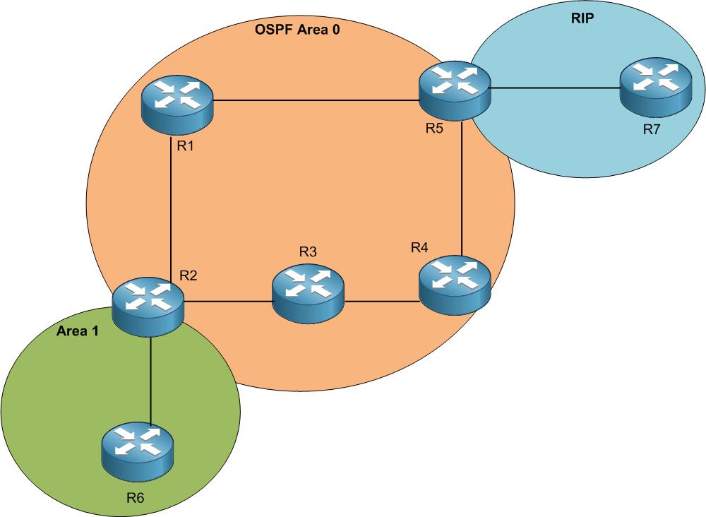
7. Example Scenario
- Area 0 → Core network
- Area 1 → Branch office
- Area 2 → Another branch
All communication between Area 1 and Area 2 goes through Area 0.


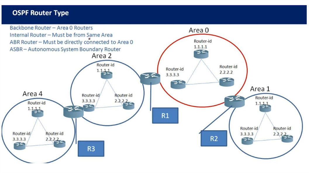
OSPF Router Types
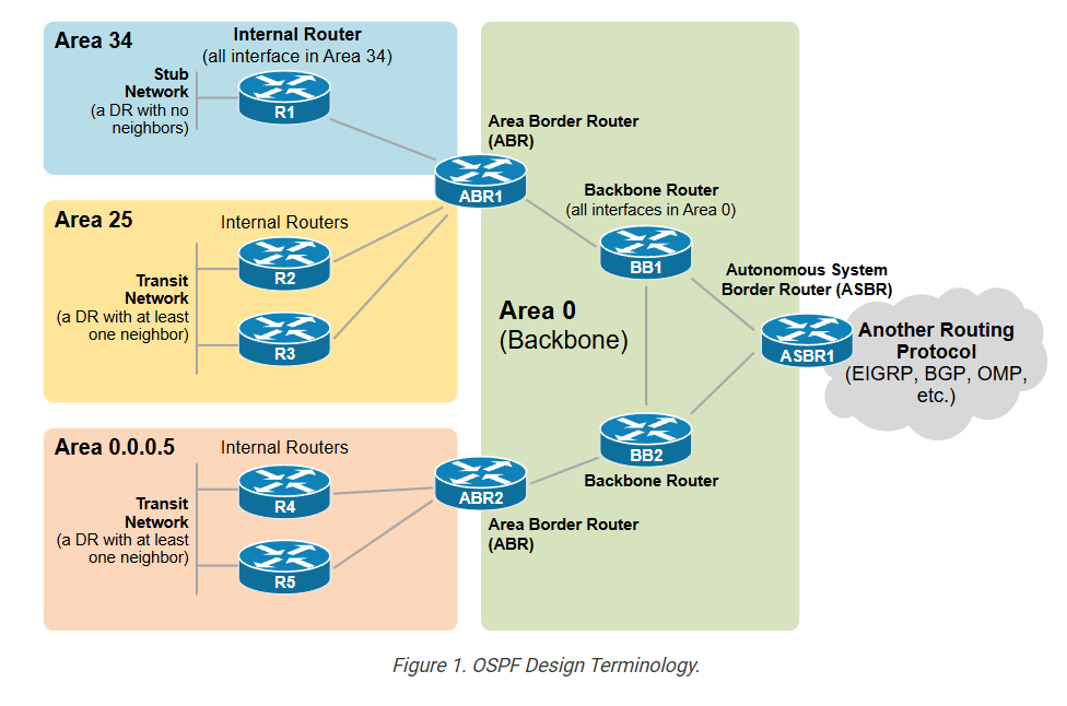
1. Overview of OSPF Router Types
In OSPF (Open Shortest Path First), routers are divided into different types based on their location and role in the network topology. This classification helps OSPF manage routing efficiently in both small and large (multi-area) networks. Each router type has a specific function in maintaining the Link-State Database (LSDB) and forwarding traffic.
2. Internal Router
An Internal Router is a router whose all interfaces belong to the same OSPF area. It only participates in routing within that single area and maintains one LSDB.
👉 Working:
It exchanges routing information only with routers in the same area and does not deal with inter-area or external routes.
👉 Example:
A router with all interfaces in Area 1 is an Internal Router.
👉 Key Points:
- Single area only
- Simple design
- Generates Type 1 LSA (Router LSA)
3. Backbone Router
A Backbone Router is any router that has at least one interface in Area 0 (Backbone Area). Area 0 is the central part of OSPF, and all inter-area communication must pass through it.
👉 Working:
It helps carry routing information between different areas through the backbone.
👉 Example:
A router connected to Area 0 (even if also connected to another area) is a Backbone Router.
👉 Key Points:
- Must be connected to Area 0
- Supports inter-area communication
- Generates Type 1 LSA
4. ABR (Area Border Router)
An ABR (Area Border Router) is a router that connects Area 0 with one or more other areas. It is responsible for exchanging routing information between areas and maintaining separate LSDBs for each area.
👉 Working:
ABR summarizes routes and sends them between areas to reduce routing table size and improve performance.
👉 Example:
- Interface 1 → Area 0
- Interface 2 → Area 1
→ Router becomes ABR
👉 Key Points:
- Connects multiple areas
- Maintains multiple LSDBs
- Generates:
Type 1 LSA
Type 3 (Summary LSA)
Type 4 (ASBR Summary LSA)
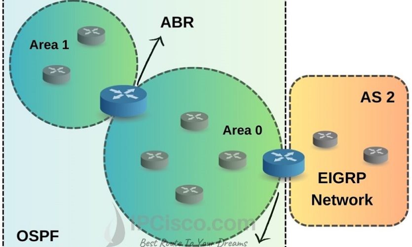
5. ASBR (Autonomous System Boundary Router)
An ASBR is a router that connects OSPF with external networks or other routing protocols such as static routes, RIP, EIGRP, or BGP.
👉 Working:
It redistributes external routes into OSPF so that other routers can reach networks outside the OSPF domain.
👉 Example:
A router connected to the internet and redistributing routes into OSPF becomes an ASBR.
👉 Key Points:
- Injects external routes
- Generates:
Type 1 LSA
Type 5 (External LSA)
Type 7 (in NSSA)
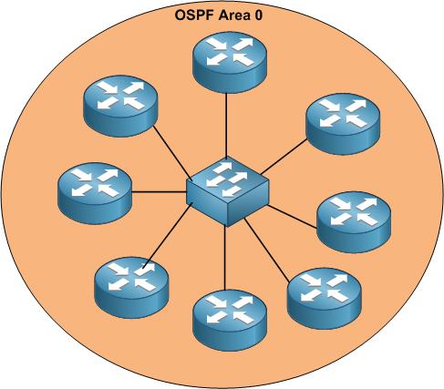
6. DR (Designated Router)
A DR (Designated Router) is elected in multi-access networks like Ethernet to reduce OSPF traffic and adjacency formation.
👉 Working:
Instead of all routers forming full mesh adjacency, all routers send updates to the DR, and the DR distributes them.
👉 Example:
In a LAN with 5 routers, one becomes DR to manage communication.
👉 Key Points:
- Reduces network traffic
- Central point for LSA exchange
- Generates Type 2 LSA (Network LSA)
7. BDR (Backup Designated Router)
A BDR (Backup Designated Router) is the backup of the DR. It listens to all OSPF updates and takes over if the DR fails.
👉 Working:
If the DR goes down, BDR immediately becomes DR without re-election delay.
👉 Example:
In a LAN, second-highest priority router becomes BDR.
👉 Key Points:
- Provides redundancy
- Improves network stability
- Does not generate Type 2 unless it becomes DR
8. Summary Table
| Router Type | Role | LSA Generated |
|---|---|---|
| Internal Router | Single area | Type 1 |
| Backbone Router | Area 0 | Type 1 |
| ABR | Connects areas | Type 1, 3, 4 |
| ASBR | External routes | Type 1, 5, 7 |
| DR | Central in LAN | Type 2 |
| BDR | Backup of DR | (None normally) |
- Router A → Internal Router
- Router B → ABR + Backbone Router
- Router C → ASBR
- DR/BDR → Used if LAN present
Final Conclusion
- Internal Router → Works inside one area
- Backbone Router → Connects to Area 0
- ABR → Connects multiple areas
- ASBR → Connects external networks
- DR/BDR → Optimize LAN communication
OSPF Table

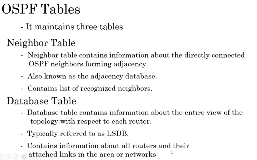
1. Overview
OSPF (Open Shortest Path First) is a link-state routing protocol that uses three main tables to operate efficiently. These tables help OSPF discover neighbors, build network topology, and calculate the best path for data forwarding. The three tables are:
- Neighbor Table (Adjacency Database)
- Topology Table (Link-State Database – LSDB)
- Routing Table (Forwarding Table)
Each table has a specific role and works together in a step-by-step process.
OSPF maintains three tables
Neighbor Table : Neighbor table contains information about the directly connected ospf neighbors forming adjacency
Database table : contains information about the entire view of the topology with respect to each router.
Routing information Table: Routing table contains information about the best path
calculated by the shortest path first algorithm in the database table.
2. Neighbor Table (Adjacency Database)
The Neighbor Table stores information about all directly connected OSPF neighbors. Routers discover neighbors using Hello packets. When parameters match (Area ID, Hello/Dead timers, authentication, etc.), they form adjacency.
👉 What it contains:
- Neighbor Router ID
- Neighbor IP address
- State (Down, Init, 2-Way, Full, etc.)
- DR/BDR information
- Interface used
👉 Working:
When a router sends Hello packets, it checks if the neighbor responds. If successful, they move through states (Init → 2-Way → Full) and become fully adjacent.
👉 Purpose:
- Maintains neighbor relationships
- Ensures communication between routers
- Required before exchanging LSAs
Commnd
show ip ospf neighbor
3. Topology Table (Link-State Database – LSDB)
The Topology Table, also called the LSDB, stores all Link-State Advertisements (LSAs) received from all routers in the same area. It represents a complete map of the network topology.
👉 What it contains:
- Type 1 → Router LSA
- Type 2 → Network LSA
- Type 3 → Summary LSA
- Type 4 → ASBR Summary LSA
- Type 5 → External LSA
- Type 7 → NSSA LSA
👉 Working:
Each router floods LSAs to neighbors. These LSAs are stored in the LSDB. All routers in the same area must have identical LSDBs.
👉 Purpose:
- Builds full network topology
- Used by SPF algorithm to calculate shortest path
👉 Command:
show ip ospf database
4. Routing Table (Forwarding Table)
The Routing Table contains the best routes selected by the SPF (Shortest Path First) algorithm. It is the final table used to forward packets.
👉 What it contains:
- Destination network
- Next-hop IP address
- Outgoing interface
- Metric (cost)
- Route type (O, O IA, O E1, O E2)
👉 Working:
After LSDB is built, the router runs SPF algorithm to calculate the shortest path. Only the best routes are installed in the routing table.
👉 Purpose:
- Used for actual packet forwarding
- Stores optimized paths
👉 Command:
show ip route ospf
5. How All Three Tables Work Together
👉 Step-by-step process:
- Neighbor Table → Routers discover and form adjacency
- LSDB (Topology Table) → Routers exchange LSAs and build full network map
- SPF Algorithm → Calculates shortest path
- Routing Table → Best routes installed for forwarding
6. Real Example
- Router A connects to Router B
- They exchange Hello packets → Added in Neighbor Table
- They exchange LSAs → Stored in LSDB
- SPF runs → Calculates best path
- Best route added → Routing Table
7. Key Differences
| Table | Function | Data Type | Usage |
|---|---|---|---|
| Neighbor Table | Stores neighbors | Router info | Adjacency |
| LSDB | Stores topology | LSAs | Path calculation |
| Routing Table | Stores best path | Routes | Packet forwarding |
Final Conclusion
- Neighbor Table → Who are my neighbors
- LSDB → Complete network map
- Routing Table → Best path for data
👉 These three tables are the core foundation of OSPF operation and are very important for troubleshooting and interviews.
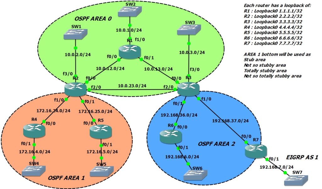
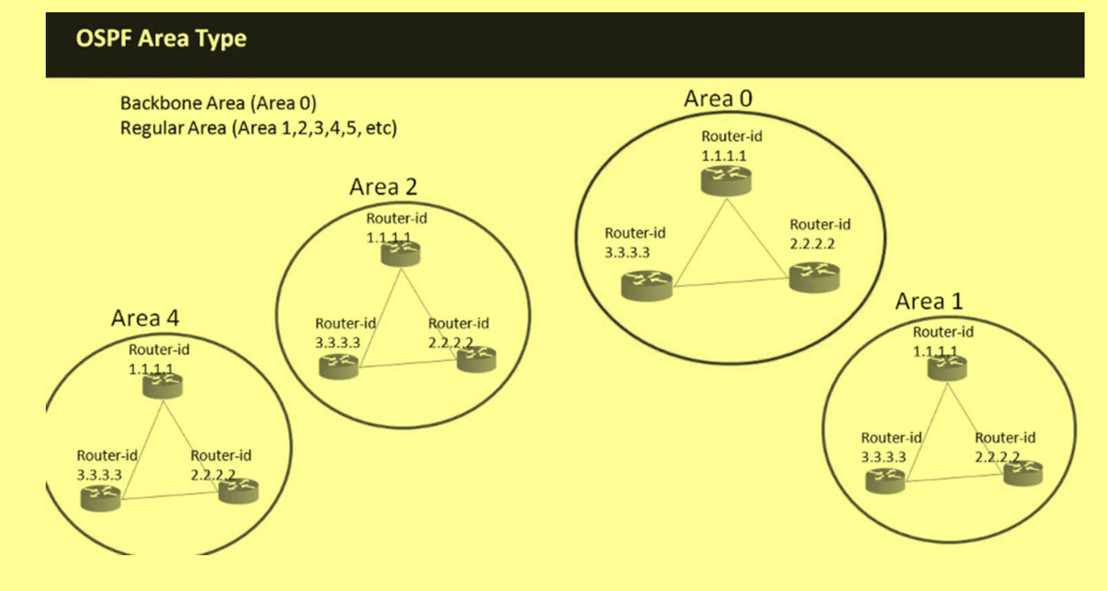
OSPF Area Types
1. Overview of OSPF Area Types
In OSPF (Open Shortest Path First), areas are used to divide a large network into smaller parts. This improves performance, reduces routing overhead, and makes the network scalable. OSPF supports different area types, each designed for specific purposes.
2. Backbone Area (Area 0)
The Backbone Area (Area 0) is the most important area in OSPF. All other areas must connect to Area 0 directly or through a virtual link.
👉 Working:
It carries inter-area routing information between different areas.
👉 Key Points:
- Mandatory in OSPF
- Handles all inter-area communication
- Supports all LSA types
3. Normal Area
A Normal Area is a standard OSPF area that allows all types of LSAs.
👉 Working:
- Receives intra-area, inter-area, and external routes
- No restrictions on LSAs
👉 LSA Allowed:
Type 1, 2, 3, 4, 5
👉 Use Case:
- Default area type
- Used in most networks
4. Stub Area
A Stub Area is used to reduce routing table size by blocking external routes.
👉 Working:
- Blocks Type 5 LSAs (External routes)
- Receives a default route (0.0.0.0) from ABR
👉 LSA Allowed:
Type 1, 2, 3
👉 Key Points:
- No ASBR allowed inside
- Reduces memory and CPU usage
👉 Command:
area 1 stub
5. Totally Stubby Area (Cisco)
A Totally Stubby Area is a more restrictive version of a stub area.
👉 Working:
- Blocks Type 3 and Type 5 LSAs
- Only allows a default route
👉 LSA Allowed:
Type 1, 2
👉 Key Points:
- Very small routing table
- Used in branch offices
👉 Command:
area 1 stub no-summary
6. NSSA (Not-So-Stubby Area)
An NSSA allows external routes inside a stub-like area.
👉 Working:
- Blocks Type 5 LSAs
- Allows external routes as Type 7 LSAs
- ABR converts Type 7 → Type 5
👉 LSA Allowed:
Type 1, 2, 3, 7
👉 Key Points:
- Supports ASBR inside the area
- Useful when external routing is required
👉 Command:
area 1 nssa
7. Totally NSSA Area
A Totally NSSA Area is an advanced version of NSSA with more restrictions.
👉 Working:
Blocks Type 3 and Type 5 LSAs
Allows only:
Type 7 LSAs
Default route
👉 LSA Allowed:
Type 1, 2, 7
👉 Key Points:
- Minimal routing table
- Used in branch networks with external routes
👉 Command:
area 1 nssa no-summary
8. Summary Table
| Area Type | Type 3 | Type 5 | Type 7 | Default Route |
|---|---|---|---|---|
| Normal | Yes | Yes | No | No |
| Stub | Yes | No | No | Yes |
| Totally Stubby | No | No | No | Yes |
| NSSA | Yes | No | Yes | Optional |
| Totally NSSA | No | No | Yes | Yes |
Final Conclusion
- Normal Area → No restriction
- Stub → Blocks external routes
- Totally Stubby → Only default route
- NSSA → Allows limited external routes
- Totally NSSA → Minimal + external support

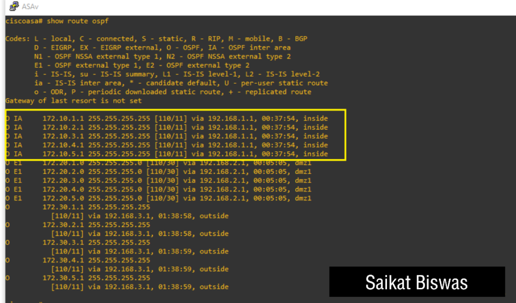
OSPF Route Codes
1. Overview
In OSPF, route codes are shown in the routing table (show ip route) to identify how a route is learned and its type. These codes help network engineers understand whether a route is internal, inter-area, or external.
2. O (Intra-Area Route)
O indicates that the route is learned from within the same OSPF area.
👉 Working:
Routers exchange LSAs inside the same area, and SPF calculates the shortest path.
👉 Key Points:
- Uses Type 1 & Type 2 LSAs
- Most preferred OSPF route
- Fast and efficient
👉 Example:
Router in Area 1 learns route from another router in Area 1
3. O IA (Inter-Area Route)
O IA means the route is learned from another OSPF area through an ABR (Area Border Router).
👉 Working:
ABR sends summary routes between areas using Type 3 LSA.
👉 Key Points:
- Uses Type 3 LSA
- Less preferred than intra-area
- Requires Area 0 backbone
👉 Example:
Router in Area 1 learns route from Area 0
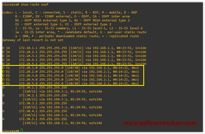
4. O E1 (External Type 1 Route)
O E1 is an external route redistributed into OSPF and calculated using both internal and external cost.
👉 Working:
Total cost = cost inside OSPF + cost from external network
👉 Key Points:
- Uses Type 5 LSA
- More accurate path calculation
- Preferred over E2
👉 Example:
Static route redistributed into OSPF with metric-type 1
5. O E2 (External Type 2 Route)
O E2 is also an external route, but it uses only external cost for path calculation.
👉 Working:
Internal OSPF cost is ignored
👉 Key Points:
- Default external route type
- Uses Type 5 LSA
- Less accurate than E1
👉 Example:
Internet route injected into OSPF
6. O N1 (NSSA External Type 1)
O N1 is an external route inside an NSSA area, calculated using both internal and external cost.
👉 Working:
Similar to E1 but used in NSSA
👉 Key Points:
- Uses Type 7 LSA
- Converted to Type 5 by ABR
7. O N2 (NSSA External Type 2)
O N2 is an NSSA external route using only external cost.
👉 Working:
Similar to E2 but inside NSSA
👉 Key Points:
- Uses Type 7 LSA
- Default type in NSSA
8. Route Preference Order
OSPF prefers routes in this order:
- O (Intra-area) → Best
- O IA (Inter-area)
- O N1 / O E1
- O N2 / O E2